FLDR? I Barely Even Know Her!
- Published on
- ∘ 24 min read ∘ ––– views
Previous Article
Next Article
Introduction
Fellas, you ever just want to sample from a discrete distribution in optimal space and time complexity?
All the time – right?!
In this edition of Peader's Digest we'll take a look at a paper from a couple years ago about this very subject:
"The Fast Loaded Dice Roller: A Near-Optimal Exact Sampler for Discrete Probability Distributions."
When I first stumbled across this paper, I think I was literally scrolling through arXiv, raw. Like riding the high of a good TV show which which has come to a conclusion, and browsing Netflix for the next binge, I was looking for something flashy.

At the time, I thought I got got. Despite a handful of neat diagrams, I was mostly puzzled by the contents, conclusion, and even the initial question being investigated in the first place. I was doubly stricken with idkwtf-this-is-ism when I looked to the source code and was faced with variable names of a single letter.
(thoughts on un-obvious variable names of a single character)

I had printed it out for something to read during a long flight, struggled through it to the best of my ability, and forgot about it entirely until earlier this week (2 years and some change later) when I realized that much of the CRDT paper2 that also went over my head when I first encountered it years ago was now rather comprehensible.
The point being that it is important for me to regularly read things that I don't understand. Eventually3 I might return to one such challenging piece of literature with greater appreciation, equipped with even just a few more semesters or years worth of exposure to the subjects which I once found alien. The digest and examination4 of a selection the algorithms described in the paper are the focus of this post.
As with many of my posts in the past couple years, much of the contents are for my own edification, as a more-public form expression rubber-duckying5 my way through things I'm trying to teach myself, while hopefully also providing some occasionally insightful or humorous commentary along the way.
Motivation: Men Who Stare at Lava Lamps
So, why the hell would we want a Fast Loaded Dice Roller? At first glance, it almost seems like a glorified inspection of /dev/random. Smarter people than I6,7,8 have written about pseudo-random number generation at length and how incorporating uncertainty can help machines make human-like predictions to improve simulation of phenomena that rely on probabilistic decision making.
However, encoding probability distributions to be sampled according to a PRG is either a time- or space-expensive exercise. Entropy optimal distribution samplers do already exist, as shown by Knuth and Yao,9 but as Saad points out:
Many applications that run quickly use a lot of memory, and applications that use little memory can have a long runtime. Knuth and Yao’s algorithm falls into the first category, making it elegant but too memory-intensive for any practical use.
The goal of their paper is to strike a balance between this trade-off, producing a more efficient sampler in terms of both time and space complexity.
The Problem
Formally, the authors present the problem as follows.
Suppose we have a list of positive integers which sum to . These integers can be thought of as weights on a loaded die. We can normalize these weights to get a probability distribution .
The goal is to construct a sampler (a die) for discrete distributions with rational entries, like our .
Sampling in this manner is a fundamental operation in many fields and has applications in climate modeling, HFT, and (most recently [for me]) fantasy Smite Pro League drafting. Existing models for sampling from a non-uniform (weighted) discrete distribution have been constrained by the prohibitive resources required to form the encode and sample from
Understanding Knuth and Yao's Optimal DDG
A random source lazily (as needed) emits or , which can be interpreted as fair, independent and identically distributed coin flips. For any discrete distribution , can be thought of as a partial map from the finite sequence of coin flips to outcomes.
That is, is the disjoint union of sequences of mapped to the rational entries in :
We treat as the sampling algorithm for and we can represent it as a Complete Binary Tree.
Aside: Taxonomy of a Tree
Though not exhaustive, it's worth spending a brief minute examining the structure of a tree, specifically binary trees.
Trees are a common recursive structure used throughout computer science, and those who venture outside have even claimed to see some naturally occurring trees in the wild!
Trees are a special kind of directed acyclic graph where the topmost node is referred to as a root with 0 or more children. Nodes can have many children, but the most common variety of tree, and the kind used for the samplers being discussed, are binary trees, meaning they can have at most 2 children. A node that has no children is called a leaf, and nodes with children are called internal.
A tree is said to be complete if every level of the tree, except for perhaps the deepest level, is completely filled, and all nodes are as far left as possible. This is not to be confused with a full binary tree, where every node except for the leaves have two children.
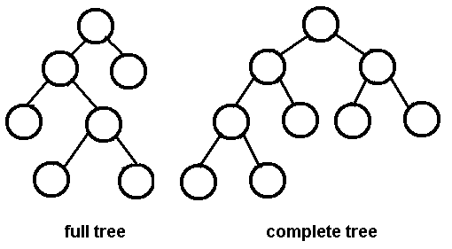
The depth of a tree is given by the length of the longest path from root to leaf. The root has a depth of 0 (since it is itself), it's children a depth of 1, and so on.

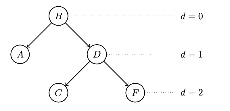
Here, is the root, is an internal node, and are leaf nodes. This tree is full, but not complete.
Tree representation
Trees can be modeled as a recursive class e.g.
class TreeNode
  def __init__(self, data):
    # references to another TreeNode mayhaps
    self.left  = None
    self.right = None

    self.data  = data
this is like straight up the laziest representation of a Tree you can imagine. There's no reason to do this in lieu of other class methods which I have not supplied.
Other, speedier representations include adjacency matrices and heaps which come with some nice properties of there own:
Graph as an Adjacency Matrix
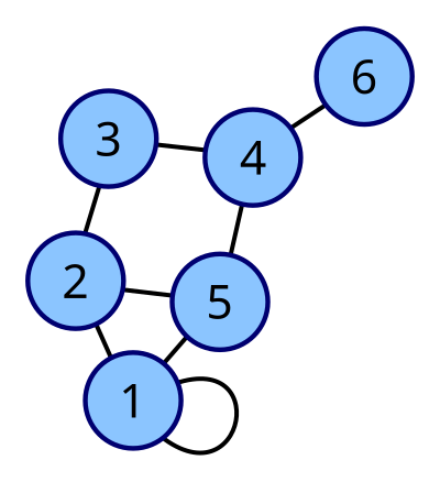
The above graph has the corresponding adjacency matrix:
where a implies an edge between node and .
Aside about Binary Expansion of Rational Numbers
Another Aside? Call that a Bside. Call that a coin.
Intuitively,10 we can convince ourselves that given a base , a rational number has a finite representation in that base iff the prime factors of the reduced denominator each divide base . So, in binary, the base of information theory, the only rational numbers with finite representations are dyadics of the form . So, unfortunately for us, most numbers will instead have infinite binary representations.
Converting from Binary to Base 10
The dyadics themselves are rather straightforward:
But for more greebled numbers, like, y'know, most of the ones we encounter outside of the memory bus, we instead have to take our binary representation, and sum the product of each digit with the corresponding power of two:
For the decimal representation of we have:
Since the geometric series
converges to , we know it's theoretically possible to build any decimal with the sum of negative powers of two via ad hoc removal of the entries of the series we don't want, yielding our decimal.
Converting from Base 10 to Binary
This process is a bit more tedious, but fundamentally the inverse of the above conversion.
We double our decimal, and whenever the resulting product is greater than , append a to our binary sequence and truncate the product, otherwise we append a :
For the binary representation of , we have:
and as noted above, this can go on for awhile: decimals with finite digits may have infinite binary expansions... The binary representations will be exact iff is the sole prime factor of the denominator which is like anti-swag.
Entropy-Optimal Sampling (Knuth and Yao)
The algorithm for sampling from a discrete distribution using a binary tree is as follows:
- Start at the root, traverse to a child according to the output of our entropy source which is accessed via primitive function
- If the child is a leaf, return its label, otherwise repeat

We call such a tree a Discrete Distribution Generating Tree (DDG).
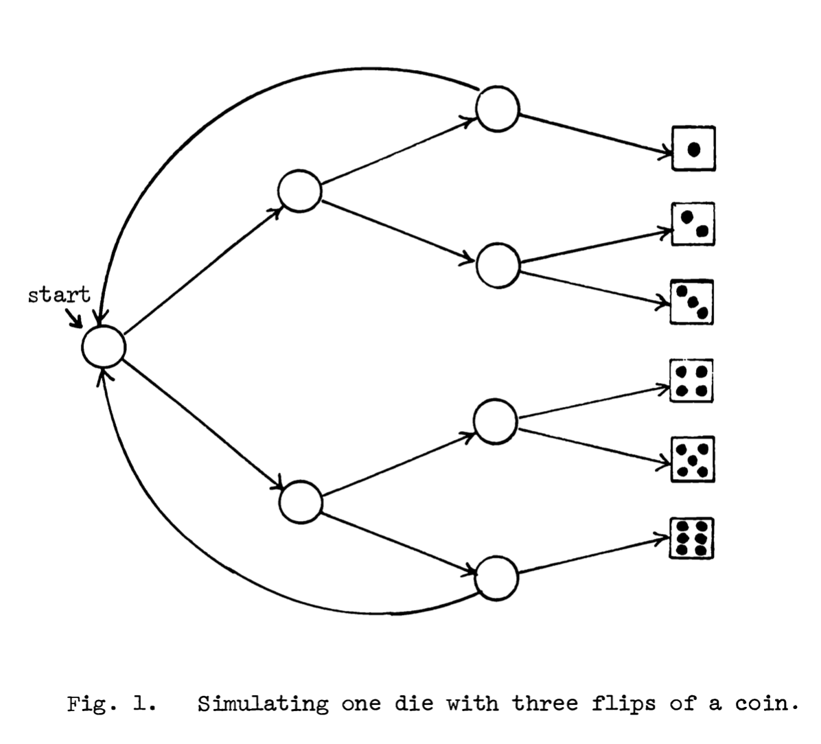
For a fair dice , we have the map from sequences of coin flips mapped to outcome of a dice roll where and are rejected and the tree is sampled again for a value in the domain of the distribution.
Back to Knuth and Yao's optimal DDG:
This begs the question, what is the entropy optimal number of flips, that is –the least, average number of flips– needed for a DDGT of some distribution ?
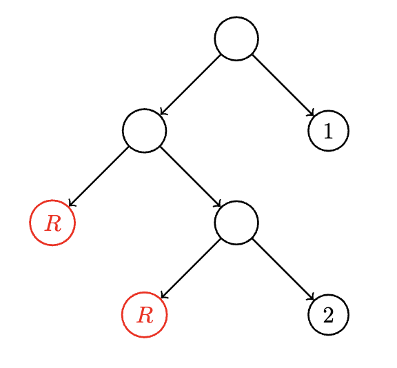
In Algorithms and Complexity: New Directions and Recent Results, Knuth and Yao present a theorem stating that the entropy-optimal tree has leaf at level iff the th bit in the binary expansion of .
For example, for the distribution
This is rather useful as it dictates precisely how we can build the optimal tree by simply reading off the binary expansion of the probabilities of our target distribution.
To construct the tree, we create a root, and two children since a die is necessarily at least two sided. For the first entry in the distribution, corresponding to the first face of our loaded die, we have . Since we need the tree to be complete, we fill from left to right. The first layer of children corresponds to , and the th digit in the binary expansion of is a 1, so we add the label to that node. and both have s in the th position of their binary expansion, but do have 1s in the th position, so we create two children whose parent is the left child of the root, and add the labels and to those leaves, yielding the following optimal tree:

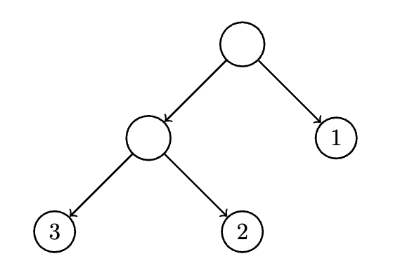
That was a rather easy and contrived example since was constructed to be dyadic, meaning all it's entries were powers of two:
But as we observed in Figure 1 above, for even just a conventional six-sided dice, non-dyadic entries become necessary to account for. This is where the caveat of "near-optimal" comes into play.
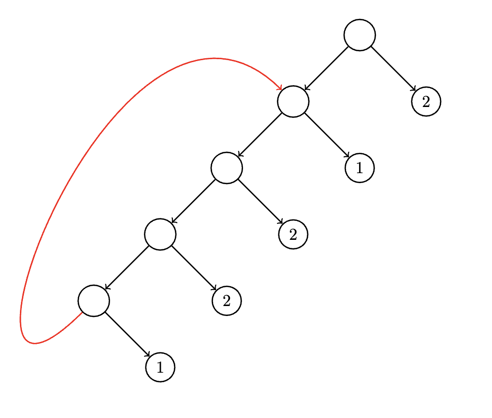
Consider instead a discrete probability with rational (aka annoying entries). The binary expansions of these entries may be infinite. But fear not, we can make use of back edges which refer back to a node at a higher depth in the tree whose descendants capture the repeating portion of the expansion:

What about discrete transcendental distributions, like
Eric Weisstein, no not that one, nor that one, but the cool one does research for Wolfram Alpha published a paper earlier this year showing that binary transcendental distributions might actually be more tractable than was previously thought: https://arxiv.org/abs/2201.12601
Knuth and Yao's theorem actually still holds for irrationals and transcendentals. However, we can't represent these on a computer with finite memory, and by definition, there's no repeating structure for irrational probabilities, so back edges can't help us out much further.
2nd Main Theorem
The second main theorem introduced by Knuth and Yao which has direct relevance to FLDR is that the expected number of flips in an entropy-optimal satisfier satisfies the following constraint:
where is the Shannon entropy or amount of information per bit. Information is inherently related to "surprise," –that is: we are unsurprised when an event occurs with probability , (duh, that's what we expected to happen), and immensely surprised when we observe an event that had probability of occurring.
The lower bound of this theorem follows from the definition of Shannon entropy –we can't receive less than one bit of information per flip.
The upper bound is less obvious, but Knuth and Yao prove that for a uniform distribution on which can be represented as a full binary tree with exactly bits, the worst case cost for sampling this distribution is 2-bits for non-full Binary Trees.
So, What's the Problem...?
Why not just use an optimal sampler as described above? Well, if you hadn't guessed already, they require a ton of memory.
In general, the sampler described above is exponentially large in the number of bits needed to encode the target distribution :
for summing to , with . To go from the logarithmic encoding of to the polynomial encoding of the KY-DDG is an exponential scaling process. In other words, to optimally encode and sample a binomial distribution with , the KY-DDG has a staggering depth of which is roughly equivalent to terrabytes. Talk about combinatorials which fry your gonads!11
FLDR, on the other hand, scales linearly with the number of bits needed to encode :

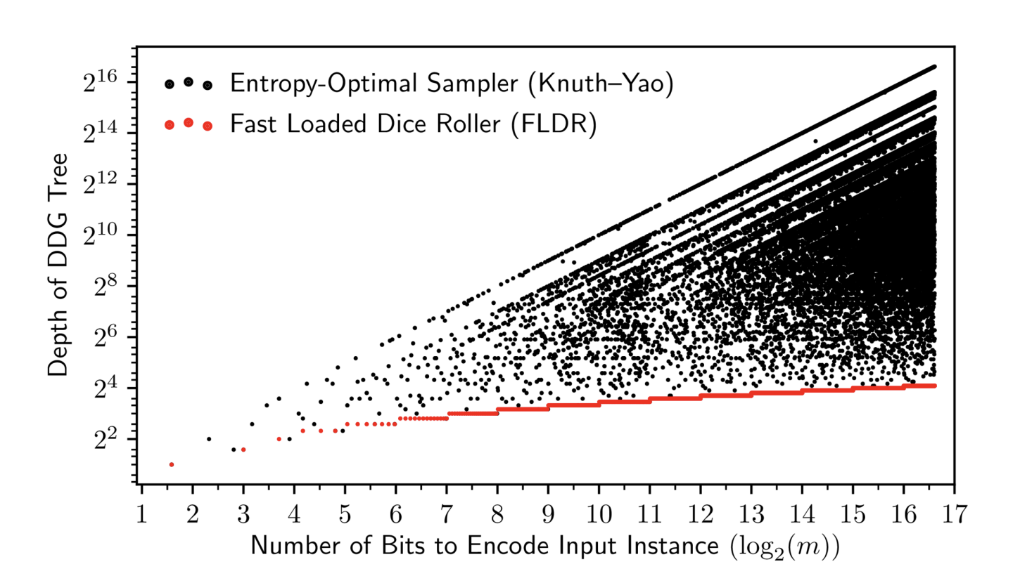
Whereas the entropy-optimal sampler is bounded by per Knuth and Yao's 2nd theorem, FLDR only increases the upper bound by 4 flips in the worst case:
with a depth given by , and boasting bits to encode both and the FLDR-DDG.
How Does FLDR Work?
The basic idea behind FLDR is rejection sampling. The advances made in reducing the encoding costs are gained from clever representation of the DDG.
A naive approach to rejection sampling might be a tabular approach like the following:
for with , build a look-up table where is represented proportionately:


where is fixed so that . To encode a distribution as such a table, generate random bits to form an integer until and return the lookup table of size to be sampled from.
This will work, but is still an exponentially sized array.
We can do a bit better by shrinking the table from size to by using inverse Cumulative Distribution Function Sampling:

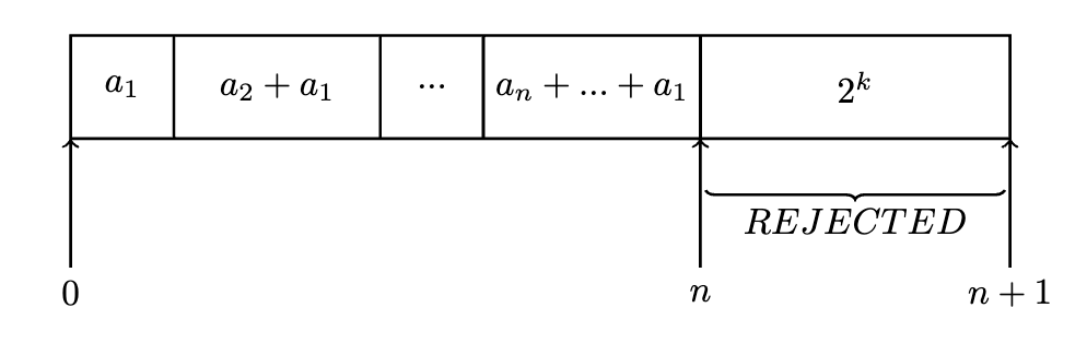
Similarly, with this approach, generate random bits to form an integer until and return
And finally, FLDR is a DDG Tree with Rejection Sampling. Once again, fixing so that , we also introduce a new distribution where and build from which is the optimal DDGT of this distribution which has been "padded" to form a dyadic distribution, where the extra entries are "rejects."

Comparing each of these approaches:
| approach | bits/sample | time complexity | space complexity |
|---|---|---|---|
| Naive Rejection Sampling | |||
| Inverse CDF | |||
| FLDR |
Results
The main advantages of FLDR over other approaches include:
- memory required scales linearly in the number of bits needed to encode
- FLDR requires 10,000 times less memory than the entropy-optimal sampler
- Rejection sampling from incurs only a 1.5x runtime penalty
- FLDR is 2x-10x faster in preprocessing
Footnotes & References
Footnotes
I will never stop using memes in my posts. In fact, every year that passes erodes the mountain of cringe that might otherwise be earned from tossing a rage comic in here... ↩
https://www.murphyandhislaw.com/blog/strong-eventual-consistency ↩
The authors of this pre-print receive 3/5 swag points from me for uploading their code along with the paper. -2 swag for said code being hard to read. An example of a paper with code that receives 5/5 swag points from Peter is "Escaping the State of Nature: A Hobbesian Approach to Cooperation in Multi-agent Reinforcement Learning"(arXiv:1906.09874) by William Long. Actually, 6/5 Will responded to me when I reached out asking about the code and later offered me a job when I was first looking for fulltime work. (The best way to earn swag points is bribery with a salary). ↩
Randomness 101: LavaRand in Production. CloudFlare ↩
Method for seeding a pseudo-random number generator with a cryptographic hash of a digitization of a chaotic system. Patent US5732138A. ↩
Recommendation for Random Number Generation Using Deterministic Random Bit Generator. NIST. ↩
Donald Knuth, Andrew Yao. "The Complexity of Nonuniform Random Number Generation." Algorithms and Complexity: New Directions and Recent Results. Traub. Were you looking for a link? I bought the last hardcopy on Amazon. Awkward... ↩
"Intuitively" is a word mathematicians use to describe their understanding of something after they've suffered an acid flash back in their kitchen ↩
https://www.murphyandhislaw.com/blog/voting-power#infertility ↩