Notes on Information Theory
- Published on
- ∘ 174 min read ∘ ––– views
Notes on Information Theory from various sources
Index
Lectures
1 | Introduction to Coding Theory
- Shannon's seminal book “A Mathematical theory of communication” (1948) measured information content in the output of a random source in terms of its entropy
- In his book, he presented the Noiseless Coding Theorem: given independent and identically distributed random variables, each with entropy ...
- can be compressed into bits with negligible loss
- or alternatively compressed into bits entailing certain loss
- Given a noisy communication channel whose behavior is given by a stochastic channel law and considering a message of bits output by a source coder, the theorem states that every such channel has a precisely defined real numbered capacity that quantifies the maximum rate of reliable communication
- Given a noisy channel with a capacity , if information is transmitted at rate (meaning message bits are transmitted in uses of the channel), then if , there exist coding schemes (encoding and decoding pairs) that guarantee negligible probability of miscommunication, whereas if , then –regardless of a coding scheme– the probability of an error at the receiver is bounded below some constant (which increases with )
- Conversely, when , the probability of miscommunication goes exponentially to 1 in
1 - A Simple Code
Suppose we need to store 64-bit words in such a way that they can be recovered even if a single bit per word gets flipped
- We could duplicate each bit at least three times, thus storing 21 bits of information per word, and limiting ourselves to roughly 1/3 of the information per word. But the tradeoff is that we could correct any single bit flip since the majority value of the three copies gives te correct value of the bit if one of them is flipped.
In 1949, Hamming proferred his code to correct 1-bit errors using fewer redundant bits. Chunks of 4 information bits get mapped to (encoded) to a codeword of 7 bits as
which can be equivalently represented as a mapping from to (operations do ) where if the column vector and is the matrix
- Two distinct 4-bit vectors get mapped to the codewords which differ in the last 3 bits (define and check that, for each non-zero , has at least 3 bits which are )
- This code can correct all single bit flips since, for any 7-bit vector, there is at most 1 codeword which can be obtained by a single bit flip
- For any which is not a codeword, there is always a codeword which can be obtained by a single bit flip
Basic Definitions
Hamming Distance
The Hamming Distance between two strings of the same length over the alphabet is denoted and defined as the number of positions at which and differ:
The fractional or relative Hamming Distance between is given by
- The distance of an error correcting code is the measurement of error resilience quantified in terms of how many errors need to be introduced to cofuse one codeword with another
- The minimum distance of a code denoted is the minimum Hamming distance between two distinct codewords of :
- For every pair of distinct codewords in , the Hamming Distance is at least
- The relative distance of denoted is the normalized quantity where is the block length of . Thus, any two codewords of differ in at least a fraction of positions
- For example, the parity check code, which maps bits to bits by appending the parity of the message bits, is an example of a distance 2 code with rate
Hamming Weight
The Hamming Weight is the number of non-zero symbols in a string over alphabet
Hamming
A Hamming Ball is given by the radius around a string given by the set
Code
An error correcting code of length over a finite alphabet is a subset of .
- Elements of are codewords in , and the collection of all the codewords is sometimes called a codebook.
- The alphabet of is , and if , we say that is -ary (binary, ternary, etc.)
- The length of codewords in is called the block length of
- Associated with a code is also an encoding map which maps the message set , identified in some canonical way with to codewords in
- The code is then the image of the encoding map
Rate
The rate of a code is defined by the amount of redundancy it introduces.
which is the amount of non-redundant information per bit in codewords of .
- The dimension of is given by
- A -ary code of dimension has codewords
Distance
- The distance of an error correcting code is the measurement of error resilience quantified in terms of how many errors need to be introduced to confuse one codeword with another
- The minimum distance of a code denoted is the minimum Hamming distance between two distinct codewords of :
- For every pair of distinct codewords in , the Hamming distance is at least
- The relative distance of denoted is the normalized quantity where is the block length of . Thus, any two codewords of differ in at least a fraction of positions
- For example, the parity check code, which maps bits to bits by appending the parity of the message bits, is an example of a distance 2 code with rate
Properties of Codes
- has a minimum distance of
- can be used to correct all symbol errors
- can be used to detect all symbol errors
- can be used to correct all symbol erasures – that is, some symbols are erased and we can determine the locations of all erasures and fill them in using filled position and the redundancy code
An Aside about Galois Fields
- A finite or Galois Field is a finite set on which addition, subtraction, multiplicaiton, and division are defined and correspond to the same operations on rationals and reals
- A field is denoted as or where is a the order or size of the field given by the number of elements within
- A finite field of order exists if and only if is a prime power , where is prime and is a positive integer
- In a field of order , adding copies of any element always results in zero, meaning tat the characteristic of the field is
- All fields of order are isomorphic, so we can unambiguously refer to them as
- , then, is the field with the least number of elements and is said to be unique if the additive and multiplicative identities are denoted respectively
- It should be pretty familiar for bitwise logic then as these identities correspond to modulo 2 arithmetic and the boolean XOR operation:
| 0 | 1 | |
|---|---|---|
| 0 | 0 | 1 |
| 1 | 1 | 0 |
| XOR | AND | ||||||||||||||||||
|---|---|---|---|---|---|---|---|---|---|---|---|---|---|---|---|---|---|---|---|
|
|
- Other properties of binary fields
- Every element of satisfies
- Every element of satisfies
3 - Linear Codes
General codes may have no structures, but of particular interest to us are a subclass of codes with an additional structure, called Linear Codes defined over alphabets which are finite fields where is a prime number in which case with addition and multiplication defined modulo .
- Formally, if is a field and is a subspace of then is said to be a Linear code
- As is a subspace, there exists a basis where is the dimension of the subspace. Any codeword can be expressed as the linear combination of these basis vectors. We can write these vectors in matrix form as the columns of an matrix call a generator matrix
Generator Matrices and Encoding
- Let be a linear code of dimension . A matrix is said to be a generator matrix for if its columns span
- It provies a way to encode a message (a column vector) as the codeword which is a linear transformation from to
- Note that a Linear Code admits many different generator matrices, corresponding to the different choices of bases for the code as a vector space
- A -ary code block of length and dimension will be referred to as an code
- If the code has distance , it may be expressed as and when the alphabet size is obvious or irrelevant, the subscript may be ommitted
Aside about Parity-Bit Check Codes
A simple Parity-bit Check code uses an additional bit denoting the even or odd parity of a messages Hamming Weight which is appended to the message to serve as a mechanism for error detection (but not correction since it provides no means of determing the position of error).
- Such methods are inadeqaute for multi-bit errors of matching parity e.g., 2 bit flips might still pass a parity check, despite a corrupted message
| data | Hamming Weight | Code (even parity) | odd |
|---|---|---|---|
| 0 | |||
| 3 | |||
| 4 | |||
| 7 |
Application
- Suppose Alice wants to send a message
- She computes the parity of her message
- And appends it to her message:
- And transmits it to Bob
- Bob recieves with questionable integrity and computes the parity for himself: and observes the expected even-parity result
- This same process works under and odd-parity scheme as well
Examples of Codes
- corresponds to the binary parity check code consisting of all vectors in of even Hamming Weight
- is a binary repetition code consisting of the two vectors
- is the linear Hamming Code discussed above
- If is the parity check matrix of the Linear Code , then is the minimum number of columns of that are Linearly Dependent
Hamming Codes Revisited
- Hamming Codes can be understood by the structure of its parity check matrix which allows us to generalize them to codes of larger lengths
- = is a Hamming Code using the Generator Matrix , and a parity matrix
and see that .
Correcting single errors with Hamming codes
- Suppose that is a corrupted version of some unknown codeword with a single error (bit flip)
- We know that by the distance property of , is uniquely determined by . We could determine by flipping each bit of and check if the resulting vector is in the null space of ,
- Recall that the nullspace of a matrix is the set of all n-dimensional column vectors such that
- However, a more efficient correction can be performed. We know that , where is the column vector of all zeros except for a single 1 in the th position. Note that the th column of which is the binary representation of , and thus this recovers the location of the error
- Syndrome: We say that is the syndrome of
Generalized Haming Codes
We define to be the matrix where column of is the binary representation of . This matrix must contain through , which are binary representations of all powers of 2 from and thus has full row rank
- The th generalized Hamming Code then is given by
and is the binary code with the parity check matrix
- Note that is an code
- Proof:
- Since has rank , and we must simply check that no two columns of are linearly dependent, and that there are three linearly dependent columns in
- The former follows since all the columns are distinct, and the latter since the first three columns of are the binary representations of 1,2,3 add up to 0.
If is a binary code of block length , and has a minimum distance of 3, then
and it follows that the Hamming Code has the maximum possible number of code words (and thus, an optimal rate) amongst all binary codes of block length and a minimum distance of at least 3.
- Proof:
- For each , define its neighbordhood of all strings that differ in at most one bit from .
- Since has distance 3, by the triangle inequality we have
yielding the desired upper bound on per this “Hamming Volume” upper bound on size of codes.
- Note that has a dimension of and therefore a size which meets the upper bound for block length
- The general definition of a Hamming or Volume Bound for binary codes of block length , and distance is given by
for equality to hold in (2), Hamming Balls of radius around the code words must cover each point in exactly once, giving a perfect packing of non-overlapping Hamming spheres that cover the full space.
- Codes which meet the bound in (2) are therefore called perfect codes
Perfect Codes
There are few perfect binary codes:
- The Hamming Code
- The Golay Code
- The trivial codes consistng of just 1 codeword, or the whole space, or the repetition code for odd
The Golay Code
Like other Hamming Codes, the Golay Code can be constructed in a number of ways. consists of when the polynomial is divisible by
in the ring .
3.3 Dual of a Code
Since a Linear Code is a subspace of , we can define its dual in orthogonal space – a co-code, if you will
- Dual Code: If is a linear code, then its dual is a linear code over over given by
where is the dot product over of vectors
- Unlike vector spaces over , where the dial (or orthogonal complement) vector of a subspace satisfies and (), for subspaces of , and can intersect non-trivially
- In fact, we can devise (a self-orthogonal code) or even just , a self-dual
3.4 Dual of the Hamming Code
The Dual of the Hamming Code has a generator matrix which is a matrix whose rows are all non-zero bit vectors of length . This yields a code and is called a simplex code
The Hadamard Code, the Hamming Code's dual, is obtained by adding an all-zeros row to
is a linear code whose generator matrix has all -bit vecotrs as its rows.
- Its encoding map encodes by a string in consisting of the dot product for every
- The hadamard code can also be dinfed over , buby encoding a message in with its dot product with ever other vector in that field
- The Hadamard Code is the most redundant linear code in which no two codeword symbols are equal in every codeword, implying a robust distance property:
- The Hadamard Code and simplex codes have a minimum distance of . The -ary Hadamard Code of dimension has a distance
- Proof: For for exactly (i.e. half) of the elemtns of .
- Assume for definiteness that .
- Then, for every , and therefore exactly one of and equals 1. The proof for the -ary case$ is similar.
- Binary codes cannot have a relative distance of more than , unless they only have a fixed number of code words. This the relative distance of Hadamard Codes is optimal, but their rate is necessarily poor
Code Families and Asymptotically Good Codes
- The Hamming and Hadamard codes exhibit two extreme trade-offs between rate and distance
- Hamming Code's rates appraochs 1 (optimal), but their distance is only 3
- Conversely, Hadamard Code's have an optimal relative distance of , but their rate approaces 0
- The natural question that follows is is there a class of codes which have good rate and good relative distance such that neither approach 0 for large block lengths?
- To answer this question, we consider asymptotic behavior of code families:
- Define a code family to be an infinite collection , where is a -ary code of block length , with and
- Many constructions of codes will belong to an infinite family of codes that share general structure and properties whoe asymptotic behavior guides their construction
- We also need extend the notion of relative rate and distance to these inifinite families:
- A -ary family of codes is said to be asymptotically good if its rate and relative distance are bounded away from zero such that there exist constant
While a good deal is known about the existence or even explicit construction of good codes as well as their limitations, the best possible asymptotic trade-off between rate and relative distance for binary codes remains a fundamental open question which has seen no improvement since the late 70s in part due to the the fundamental trade off between large rate and large relative distance
Error Correction Coding: Mathematical Methods and Algorithms - Todd Moon
1 | A Context for Error Correction Coding
1.2 - Where Are Codes
- Error Control Codes are comprised of error correction and error detection
Da heck is an ISBN
- For a valid ISBN, the sum-of-the-sum of the digits must be equal to
| digit | cum. sum | cum. sum of sum |
|---|---|---|
| 0 | 0 | 0 |
| 2 | 2 | 2 |
| 0 | 2 | 4 |
| 1 | 3 | 7 |
| 3 | 6 | 13 |
| 6 | 12 | 25 |
| 1 | 13 | 38 |
| 8 | 21 | 59 |
| 6 | 27 | 86 |
| 8 | 35 | 121 |
The final sum is
1.3 - The Communication System
Information theory treats information as a pseudo-physical quantity which can be measured, transformed, stored, and moved from place to place. A fundemental concept of information theory is that information is conveyed by the resolution of uncertainty.
Probabilities are used to described uncertainty. For a discrete random variable , the information conveyed by observing an outcome is bits.
- If , outcome of 1 is certain, then observing yields bits of information.
- Conversely, observing in this case yields ; a total surprise at observing an impossible outcome
Entropy is the average information. For our above example with a discrete, binary, random variable , we have either (entropy of the source) or (a function of the outcome probabilities) given by
- For a source having outcomes with probabilities , the entropy is
Source-Channel Separation Theorem: Treating the problems of data compression and error correction separately, rather than seeking a jointly optimal source/channel coding solution, is asymptotically optimal in block sizes
Because of redundancy introduced by the channel coder, there must be more symbols at the output of the coder than at the input. A channel coder operates by accepting a block of input symbols and outputting a block of symbols.
The Rate of a channel coder is
Channel Coding Theorem: Provided that the rate of transmission is less than the channel capacity , there exists a code such that the probability of error can be made arbitrarily small
1.4 - Binary Phase-Shift Keying
- Process of mapping a binary sequence to a waveform for transmission over a channel
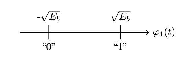
- Given a binary sequence , we map the set via
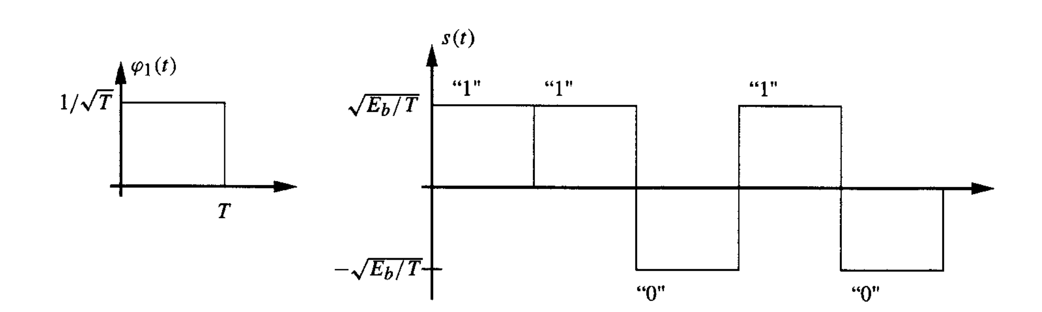
- We also have , a mapping of a bit or () to a signal amplitude which multiplies a waveform which is a unit-energy signal
over . A bit arriving at can be represented as the signal where the energy required to transmit the bit is given by
- The transmitted signal are points in a (for our purposes: one-) dimensional signal space on the unit-energy axis

such that a sequence of bits can be expressed as a waveform:

We can expand this representation to two dimensions by introducing another signal and modulating the two to establish a signal constellation. Let , for some inteeger , be the number of points in a constellation. -ary transmission is obtained by placing points in this signal space and assigning each point a unique pattern of bits.

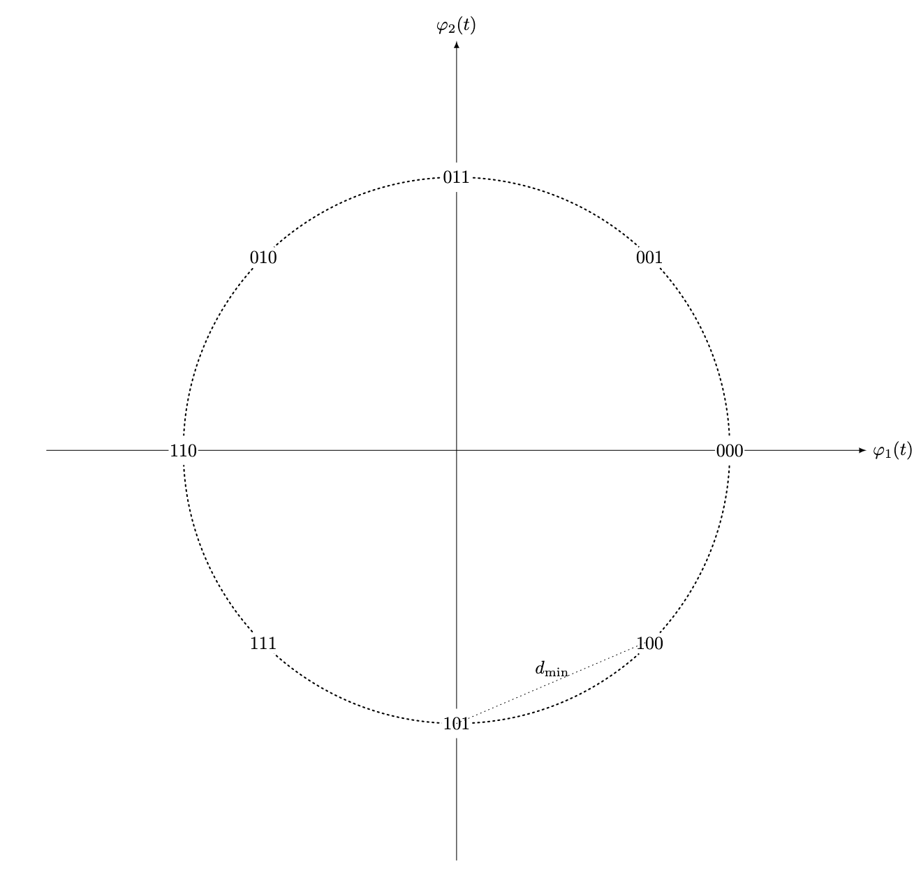
- Note that the assignment of the bits to constellation points is such that adjacent points differ by only 1 bit. Such an assignment is called Gray code order. Since it is most probably that errors will move from a point to an adjacent point, this reduces the probability of bit error
Associated with each signal (stream of bits) and signal constellation point is a signal energy
The average signal energy is the average of all signal energies, assuming that each point is used with equal probability
and ca be related to the average energy per bit
2 | Groups and Vector Space
2.1 - Introduction
Linear block codes form a group and a vector space, which is useful
2.2 - Groups
A Group formalizes some basic rules of arithmetic necessary for cancellation and solution of simple equations
A binary operation on a set is a rule that assigns to each ordered pair of elements of a set some element of the set
Since the operation is deinfed to return an element of the set, this operation is closed
We can further assume that all binary operations are closed
Examples include:
A Group is a set with a binary operation on such that
- The operator is associative: for any
- For all there exists which is the inverse of such that , where is called the identity of the group. The inverse can be denoted for multiplication-like and addition-like operations, respectively
When is obvious from context, the group may be referred to as just the set .
If has a finite number of elements, it is said to be a finite group with order , the number of elements.
A group is commutative if .
, the integers under addition, forms a group with the identity since
- The invert of . Thus the group is commutative.
- Groups with an addition-like operator are called Abelian
, the integers under multiplication, does not form a group since there does not exist a multiplicative inverse for every element of the integers.
, the rationals without zero under multiplication with the identity of and the inverse forms a group
These rules are strong enough to introduce the notion of cancellation. In a group , if , then by left cancellation via
and similarly for right hand cancellation via properties of associativity and identity.
We can also identify that solution to linear equations of the form are unique.
- Immediately, we get . If are the two solutions such that
then by cancellation, we get .
For example, let be addition on the set with the identity .
- Since appears in each row and column, every element has an inverse.
- By uniqueness of solution, we must have every element appearing in every row and column, which we do. So is a Abelian group.
One way to form groups is via the Cartesian production. Given groups , the direct product group has elements where . The operation is performed elementwise such that if
and
then
Example
The group consists of the tuplies and addition .
This is called the Klein 4-group, and intorduces the concept of permutations as elements of a group, and is a composable function as our operation as opposed to simple arithmetic groups.
Example
A permutation of set is a bijection (one to one, and onto) of onto itself. Let
then a permutation
meaning
There are different permutations on distinct elements. We can think of as a prefix operation: or . If
then
is the construction of permutations which is closed under the set of permutations with the identity and the inverse
Composition of permutations is associative: for
and thus the set of all permutations on elements forms a group under composition.
- This is known as a symmetric group on letters .
- Note that composition is not commutative since , so is a non-commutative group
2.2.1 Subgroups
A subgroup of is a group formed from a subset of elements of where indicates the relation between the two sets where is said to be a proper subgroup.
The subgroups and are the trivial subgroups.
Example
Let , both . We can show that is a group: .
Similarly,
Example
Consider the group of permutations on , which has a subgroup formed by the closed compositions:
2.2.2 Cyrclic Groups and the Order of an Element
In a group with a multiplication-like operation, we use to indicate
with being the identity element for .
For a group with additive operations is used to indicate
If , any subgroup containing must also include , etc.
It must also adhere to .
For any , the set generates a subgroup of called the cyclic subgroup. is said to be the generator of the subgroup and the resultant group is denote .
If every element of a group can be gneerated from a single element, the group is said to be cyclic.
Example
is cyclice since every element can be generated by .
In a group with , the smallest such that is equal to the identity in is said to be the order of the element .
- If no such exists, is of infinite order.
- In , 2 is of order , as are all non-zero elements of the set.
Example
If , then
Therefore is a generator for the group if and only if and are relatively prime
[IMAGE Of the planes]
2.3 - Cosets
The left coset of ( not necessarily being commutative), is the set
and the right coset is given by the symmetric relation. In a commutative group, they are obviously equal.
Let be a group, a subgroup of , and the left coset . Then, if and only f . By cancellation, we have .
To determine if are in the same (left) coset, we simply check the above condition.
Exmaple
Let and such that . Now, form the cosets:
and observe that neither are subgroups as they do not have an identity, but the union of all three cover the original group: .
We can determine whether or not two numbers are in the same coset of by checking whether
2.2.4 - Lagrange's Theorem
Basically, it's a prescription of subgroup size relative to its group.
- Every coset of in a group has the same number of elements
- Let be two elements ub tge ciset . If they are equal, then we have , and thereform the elements of a coset are uniquely identified by elements in
It follows, then, that we have the following properties of cosets:
- reflecivity: An element is in the same coset of itself
- symmetry: If are in the same coset, then are in the same coset
- transitivity: If are in the same coset, and are in the same coset, then are in the same coset as well
Therefore, the relation of "being in the same coset" is an equivalence relation, and thus, every equivalence relation partitions its elements into disjoint sets.
- It follows then that the distinct coets of in a group are disjoint
With these properties and lemmas, Lagrange's Theorem states that: If is a group of finite order, and a subgroup of , then the order of divides the order of such that . We say " divides " without remainder
- If and , then
Lagrange's Theorem implies that every group of prime order is cyclic.
- Let be of prime order, with and . Let , the cyclic subgroup generated by . Then . But by Lagrange's Theorem, the order of must ("cleanly") divide the order of . Since is prime, we must have , thus generates , so must be cyclic.
2.2.5 - Induced Operations; Isomorphism
Returning to the three sentence cosets we defined earlier, we have and define addition on as follows: for
if and only if . That is, addition of the sets is defined by representatives in the sets. The operation is said to be the induced operations on the coset: .
Taking and noting that . Similarly, via , taking the representatives to be . Based on this induced operation, we can obtain the following table
which we say is to the table for :
Two groups are said to be (group) isomorphic if there exists a one-to-one, onto function called the isomorphism such that
We denote isomorphism via . Isomorphic groups are essentially "the same thing"
Let be a group, a subgroup, and the set of cosets in . The induced operation between cosets is defined by if and only if for any provided that the operation is well-defined (no ambiguity for those operands).
For any commutative group, the induced operation is always well-defined, otherwise only for normal groups
- A subgroup of is normal if . All Abelian groups are normal.
If is a subgroup of a commutative group the induced operation on the set of cosets of satisfies
The group formed by the cosets of in a commutative (or normal subgroup) group with the induced operation is said to be the factor group of , denoted and the cosets are called the residue classes of
- We could express and in general .
A Lattice is formed by taking all the possible linear combination of a set of basis vectors. That is are a set of linearly independent vectors. A lattive is then formed from the basis by
e.g. the lattice formed by is the set of points with the integer coorinates in the plane denoted .
For the lattice , let be a subgroup with the cosets
and

2.2.6 - Homomorphism
A homomorphism is a weaker condition than the structural and relational equivalence defined by an isomorphism. A homorphism exists when sets have when sets have the same algebraic structure, but they might have a different number of elements.
The groups are said to be homomorphic if there exists a function. (not necessarily one to one) called the homomorphism such that:
Example
Let , and . For , we have
This are homomorphic though they clearly have different orders.
Let be a commutative group, a subgroup, so that is the factor group. Let be defined by , then is a homomorph known as the natural or canonical homomorphism.
The kernel of a homomorphism of a group into a group is the set of all elements of which mapped to by .
2.3 - Fields
A Field is a set of of objects on which addition, multiplication, and their inverse operations apply arithmetically (analagously to their behavior on the reals). The operations of a field must satisfy the following conditions:
- Closure under addition:
- There is an additive identity: which we denote
- There is an additive inverse (subtraction): denoted
- Additive associativity:
- Additive Commutativity:
- Closure under multiplication:
- There is a multiplicative identity: denoted such that
- Multiplicative inverse: denoted and called the reciprocal of
- Multiplicative associativity:
- Multiplicative commutativity:
- Multiplicative distribution:
The first four requirements imply that elements of form a group under addition and, with the fifth requirement, commmutativity is obtained. The latter conditions imply that the non-zero elements form a commutative group under multiplication.
Like the shorthand for groups, a field may be referred to as just , and the order of the field may be subscripted as well: a field with elements may be denoted .
Example
The field and has the following operation tables which are of particular importance for binary codes:
| XOR | AND | ||||||||||||||||||
|---|---|---|---|---|---|---|---|---|---|---|---|---|---|---|---|---|---|---|---|
|
|
The notion of isomorphism and homomorphism also exist for fields.
Two fields are (field) isomorphic if there exists a bijection such that :
For example, the field is isomorphic to ddefined above via
Lastly, fields are homomorphic if such a structure-preserving map exists which is not necessarily bijective.
2.4 - Linear 👏 Algebra 👏 Review
Let be a set of elements called vectors and be a field of element called scalars. The additive operator is defined element-wise between vectors, and scala multiplication is defined such that for a scalar and a vector
Then, is a vector space over if the additive and multiplicative operators satisfy the following conditions:
- forms a commutative group under addition
- For any elements . This also implies by (1) that we must have for all
- Addition and multiplication are distributive: and
- The multiplicative operation is associative:
Then, is called the scalar field of the vector space .
Examples
- The set of -tuples together with the elements denoted with element-wise addition:
and scalar multiplication:
- The set of -tuples with elements forms a vector space denoted with elements. For , the space is completely defined:
- And, in general, the set of tuples with the field , element-wise addition, and scalar multiplication constitutes a vector space.
A Linear Combination is just the application of these operations in a vector space:
We observe that the linear combination can be obtained by stacking the vectors as columns:
and taking the prdouct with the column vector of scalar coefficients:
Spanning Set: Let be a vector space. A set of vectors is said to be a spanning set if every vector can be expressed as a linear combination of vectors in . That is, , there exists a set of scalars such that . The set of vectors obtained from every possible linear combinations of such vectors in is called the span of , aptly denoted .
If we treat as a matrix whose columns are the vectors ,
- is the set of linear combinations of the columns of
- the column space of is the space obtained by the linear combinations of 's columns
- and similarly, the row space of of is the space obtained by the linear combinations of 's rows
If there are redundant vectors in the spanning set, not all are needed to span the space as they can be expressed in terms of other vectors in the spanning set – the vectors of the spanning set are not linearly independent.
A set of vectors is said to be linearly dependent if a set of scalars exists with not all such that their linear combination
Conversely, a set of vectors is said to be linearly independent if a set of scalars exists such that
then it must be the case that .
The spanning set for a vector space that has the minimum possible number of vectors is caleld the basis for . The number of vectors in a basis for is said to be the dimension of .
It follows that the vectors in a basis must be linearly independent, else it would be possible to form a smaller set of vectors.
example
Let , the set of binary 4-tuples and let be a set of set of vectors with
Observe that is a spanning set for , but not for all of . is not a basis for as it has some redundancy in it since the third vector is a linear combination of the first two:
and the vectors in are not linearly independent, so the third vector in can be removed, resulting in the set:
which does have .
Notice that no spanning set for has fewer vectors in it than , so .
- Let be a -dimensional vector space defined over a finite scalar field. The number of elements in , denoted . Since every vector can be written as
the number of elements in is the number of distinct -tuples that can be formed, which is .
- Let be a vector space over a scalar field , and let be a vector space. For any
for any . Then, is said to be a vector subspace of .
- Let be vectors in a vector space where . The inner product is a function of two such vectors which returns a scalar, expressed as and defined:
from which we can verify the following properties:
- Commutativity:
- Associativity:
- Distributivity:
The inner or dot product is used to describe the notion of orthogonality: two vectors are said to be orthogonal if
indicated .
Combined with the notion of vector spaces, we get the concept of a dual space. If is a -dimensional subspace of a vector space , the set of all vectors which are orthogonal to all vectors of is the orthogonal complement, dual space, or null space denoted , given by
Example
Let and
and . This example gives way to the following theorem:
Let be a finite-dimensional vector space of -tuples, , with a subspace of dimension . Let be the dual of , then
Proof
Let be a basis for such that , a rank matrix such that the dimension of the row and column spaces are both . Any vector is of the form .
Any vector must satisfy .
Let be a basis for extended to the whole -dimensional space. Every vector in the row space of is expressed as for some .
But since spans , must be a linear combination of these vectors:
so a vector in the row space of can be written
from which we observe that the row space of is spanned by the vectors
The vectors are in , so for . The remaining vectors remain to span the -dimensional row space of . Hence we must have .
Furthermore, these vectors are linearly independent because if there is a set of coefficients then
but the vectors are not in , so we must have
and since are linearly independent, we must have therefore it must be the case that
so .
3 | Linearly Block Codes
3.1 - Basic Definitions
A Block Code over an alphabet of symbols is a set of -vectors called codewords or code vectors
- An -tuple is: with elements
Associated with the code is an encoder which maps a message, a -tuple , to its associated word. To be correctively useful, we desire a one-to-one correspondence between a message and its codeword for a given code , and there might be several such mappings.
Block codes can be exhaustively represented, but for large , this would be prohibitively complex to store and decode. This complexity can be reduced by imposing structure on the code, the most common such structure being linearity.
A block code over a field of symbols with length and codewords is a -ary Linear Block Code if and only if its codewords form a -dimensional vector subspace of the vector space of all the -tuples .
- is said to be the length of the code
- is the dimension of the code
- is the proportional rate of the code
For a linear code, the sum of any two codewords is also a codeword. Furthermore, and linear combination of codewords is a codeword.
The Hamming Weight of a codeword is the number of non-zero components (usually bits) of the codeword.
- The minimum weight of a code is the smallest Hamming weight of any non-zero codeword:
For any linear code , the minimum distance satisfies . That is, the minimum distance of a linear block code is equal to the minimum weight of its non-zero codewords.
This can be proved by translating the difference of two codewords (a linear combination, and thus another codeword) "to the origin":
- As an aside, I don't love the degeneracy of the notation here, so I'm just going to scrap it and use to denote weight from here on out
An code with minimum distace is denoted . The random error correcting capability of a code with is
3.2 - Generator Matrix Description of Linear Block Codes
Since a linear block code is a -dimensional vector space, there exist linearly independent vectors which are designated such that every codeword can be represented as a linear combination of these vectors:
Considering \mathbf g_i as row vectors and stacking them, form a matrix :
and let such that . Thus, every codeword has a representation for some vector . Since the rows of (generate) span the linear code , gets its name as a Generator Matrix for the code .
can be understood as the encoding operation for the code and thus only requires storing vectors of length (rather than the vectors that would be required to store all the codewords of a non-linear code).
Note that the representation provided by is not unique, as we can devise another via row operations consisting of non-zero linear combinations such that an encoding maps to a codeword in which is not necessarily the same one obtained by .
For the Hamming code (used as an example for the rest of this section), we have the following generator matrix:
such that to encode a message , we add the first and fourth rows of to obtain .
Another generator can be used by replacing such that which is a different codeword than the original .
Let be an be a (not-necessarily linear) block code. An encoder is systematic if message symbols may be found explicitly and unchanged in the codeword such that for coordinates . (which are typically sequentially defined: ) such that .
Note that the systematicism is a property of the encoder, not the code itself. For a linear block code, the encoding operation defined by is systematic if an identity matrix can be identified among the rows of . (Neither in the example above are systematic).
A systematic generator is often expressed:
where is the identity matrix and is an matrix which generates parity symbols. The encoding operation is then .
The codeword is divided into two components:
- The part which consists of the message symbols
- The part which consists of parity check symbols
Elementary row operations do not change the rowspan, so the same code is produced. However, interchanging the columns corresponds to a change in the positions of the message symbols, so the resultant code bits are also swapped, but the distance structure of the code on the whole is preserved.
Two linear codes which are the same except for some permutation of the components of the code are said to be equivalent. Let and be generator matrices of equivalent codes. Then are related by:
- Columnal permutation
- Elementary row operations
Given any arbitrary , it is possible to put it into the form above via Gaussian elimination and pivoting.
Example
For of the Hamming code used before, an equivalent generator matrix in systematic form is :
and for the Hamming code with this generator, let the message with the corresponding codeword . Then, the parity bits are obtained via:
And the systematically encoded bits are:
3.3 - Parity Check Matrix for Dual Codes
Since a linear code is a -dimensional vector subspace of , then there must be a dual space to of dimension . The dial space to an code of is the dual code of , denoted .
- It is possible for a code to exist
As a vector space, has a basis which can be denoted by , with a matrix using these basis vectors as rows:
which is known as the parity check matrix for . This parity check matric and generator matrix for a code satisfy . The parity check matrix also has the following important property:
Let be a linear code over and be a parity check matrix for . A vector is a codeword if and only if . That is, the codewords in lie in the (left) nullspace of .
Example
For the systematic generator above, the parity check matrix is
and it can be verified that . Fruthermore, even though is not in systematic form, it still generates the same code such that . is a generator matrix for a code, the dual to the Hamming Code.
This condition imposes linear constraints among the bits of called the Parity Check Equations.
The parity check matrix above yields
The parity check matrix for a code (systematic or not) provides information about the minimum distance of the code.
Let a linear block code have a parity check matrix . The minimum distant of is equal to the smallest positive number of columns of which are linearly dependent. That is, all combinations of columns are linearly independent, so there is some set of columns which are linearly dependent.
Example
For the parity check matrix of , the parity check condition is:
The first, second, and fourth rows of are linearly dependent, and no fewer rows of are linearly dependent.
3.3.1 - Simple Bounds on Block Codes
The Singleston Bound: the minimum distance for an linear code is bounded by .
Proof: An linear code has a parity check matrix with linearly idnependent rows. Since the row rank of a matrix is equal to its column rank, . Any collection of columns must therefore be linearly dependent. Thus, the minimum distance cannot be larger than .
- A code for which the minimum distance is is called a Maximum Distance Separable code.
Hamming Spheres
A roud each code "point" is a cloud of points corresponding to non-codewords. For a -ary code, there are vectors at Hamming distance of 1 away from the codeword,
vectors at Hamming distance 2, and
vectors at distance from the codeword.
Let be a code of length over , so . Then the vectors at a Hamming distance of 1 from the codeword are:
The vectors are Hamming distance less than or equal to away from a codeword from a sphere "sphere" called the Hamming Sphere of radius . The number of codewords in a Hamming sphere up to radius for a code length over alphabet of symbols is denoted .
The bounded distance decoding sphere of a codeword is the Hamming sphere of radius
around that codeword. Equivalently, a code whose random error correction capability is must have a minimum distance between codewords satisfying .
The redundancy of a code is the number of parity symbols in a codeword: where is the number of codewords. For a linear code, we have
Hamming Bound
A -random error correcting -ary code must have redundancy satisfying .
Proof: Each of spheres in has radius with no overlap, esle it would not be possible to decode errors. The total number of points enclosed by the spheres must be less than or equal to , thus
from which the result follows from taking from both sides.
A code satisfying this bound with equality is said said to be a perfect code, a designation of how the points fall into the spheres rather than the performance of the code. The entire set of perfect codes is:
- The set of all -tuples with minimum distance of 1, with
- Odd-length binary repetition codes
- Linear Binary Hamming codes or other non-linear codes with equivalent parameters
- The Golay code
3.4 - Error Detection and Correction Over Hard-Input Channels
Let be an -vector over and let be a parity check matric for a code . The vector is called the Syndrome of . if an only if is a codeword of , otherwise it indicates the presence of error in the intended codeword .
3.4.1 - Error Detection
Suppose codeword in a binary linear block code over is transmitted through a channel and that the -vector is received. We write , where is the error vector hopefully equal to the zero vector. However, the received vector could be any vector in , since any error pattern is possible. If is the parity check matrix for , then the syndrome is given by
and if is a codeword. If , then an error has been detected.
3.4.1 - Error Detection: the Standard Array
Using Maximum Likelihood Detection, decoding a vector consists of selecting the codeword closest to in terms of Hamming distance:
Let the set of codewords in the code be , where , with , and denote the set of -vectors closer to than any other codeword (with ties broken arbitrarily). The set partitions the space of -vectors into disjoint subsets. If falls into , then being closer to than any other codeword, is decoded to , so we simply must define all .
The Standard Array is a representation of the partition ; a two-dimensional array with columns being the . It is constructed by taking every codeword belonging to its own set . Writing down the set of codewords thus gives the first row of the array. From the remaining vectors in , find of smallest weight which must lie in the set since it is closest to . But
so the vector must also lie in for each , so is placed into each . The vectors are included in their respective columns of the standard array to form the second row. We continue this proecdure, selecting an unused vector of minimum weight and addint it to each codeword to form the next row, until all possible vectors have been used.
In summary:
- Write down all codewords of
- Select from remaining unused vectors of one of minimal weight . Write in the column under the all-zero codeword, then add to each codeword in turn, writing the sum in the column under the corresponing codeword
- Repeat (2) until all vectors in have been placed in the array.
Example
For , with
the codewords are:
from the remaining -tuples, one of minimum weight is selected (e.g. ), the second row is obtained by adding this to each codeword:
and proceed until all vectors are used, selecting an unused vector of minimum weight and adding it to all codewords:
The Complete Standard Array for [7, 3]
From which we can draw the following observations:
There are codeword columns and possible vectors, so there are rows in the standard array. Therefore, an code is capable of correcting different error patterns
The difference (sum over ) of any two vectors in the same row is a code vector. In a row, vectors are and , which is a codeword since linear spaces form a subspace.
No two vectors in the same row are identical, otherwise with , which is impossible.
Every vector appears exactly once in the standard array. we know every vector must appear at least once, by construction. If a vector appears in both the -th and -th row, we must have
and for , we have for some meaning is on the -th row of the array, which is a contradiction.
Rows of the standard array are cosets of the form that is, rowas are translations of the code
- Vectors in the first column are called coset leaders representing the error patterns that can be corrected by the code under this decoding strategy. The decoder in the example which the table corresponds to can correct:
- all errors of weight 1,
- seven errors of weight 2,
- and 1 error pattern of weight 3
To actually use the standard array, we locate the received error vector , the identify for some error which is a coset leader (left column) and a codeword in the top row. Since our standard array cosntruction fills the table in order of increasing error weight, the error codeword is the ML decision.
Example
Let . It's coset leader is (shown in bold in the table) which corresponds to since the generator is systematic.
Example
Not all patterns of two errors are correctable under this example code and standard array. Only seven patterns of 2, and one error of 3. Thus, the minimum distance is 4 since the weight of non-zero codewords is 4. Thus, the code is only guaranteed to be correct for error, but it does correct all of these.
A Complete Error Correcting Decoder is a decoder that, given a received word , selects codeword which minimizes . If a standard array is used as the decoding mechanism, then compelte decoding is achieved. On the other hand, if it is filled out such that up to instances of errors appear in the table, and all further rows are ommitted, the a bounded distance decoder is obtained.
A -error correcting Bounded Distance Decoder selects the codeword given the recieved vector if . If no such exists, a decoder failure occurs.
- E.g., if only rows 1 through 8 in the example standard array above were used, a in rows 9-16 would result in failure since those rows correspond to error patterns of weight 2 and 3.
A perfect code is one for which there are no "leftover" rows in its standard array; all error patterns of weight and all lighter patterns appear as coset leaders. Thus the bounded distance decoder is the ML decoder.
The obvious drawback of the standard array decoder is the memory required to express the error patterns. For a not-unreasonable binary code , the standard array would require vectors of length 256 bits to be stored, and every decoding operation would be .
The first step towards reducing storage and search complexity (still insufficient to be practical) is Syndrome Decoding. For a vector in the standard array, the syndrome is . In fact, every vector in the coset has the same syndrome, so we need only store syndromes and their associated patterns: a lookup table with rows, but only two columns, necessarily smaller than all but the trivial standard array; but still largely impractical!
Nonetheless, with such a table, we could decode:
- Compute the syndrome
- Lookup the corresponding error pattern
- Then
Example
For the code with parity check matrix
The syndrome decoding table is :
| Error | Syndrome |
|---|---|
And for , we have , so . The decoded codeword is then .
Nevertheless, additional algebraic structure must be imposed to reduce the and resource consumption of decoding techniques, as syndrome arrays still fail to sufficiently reduce the overall complexity.
3.5 - Weight Distribution of Codes and Their Duals
Let be an code, and denote the number of codewords of weight in , then the set of coefficients is called the weight distribution for the code, which is conveniently represented as a polynomial:
called the weight enumerator, which is basically the -transform of the weight distribution sequence.
Example
For the Hamming code, there is one codeword of weight 0, and the rest have weight 4, so : .
The MacWilliams Identity states that, for an linear block code over with weight enumerator , and being the weight enumerator of , then:
which allows us to characterize the dual of the code, or rearrange to characterize :
The proof of this theorem is ugly and so I left it out, but it relies on the Hadamard Transform. For a function defined on , the Hadamard Transfrom of is:
where the sum is taken over all tuples , but can be generalized to larger fields.
This gives way to the following lemma: if is an binary linear code, and is a function defined over , then
3.6 - Hamming Codes and Their Duals
For any integer , a binary code may be defined by its parity check matrix , which is obtained by enumerating all possible binary representations of in order. Codes which follow this structure are called Hamming Codes.
Example
For , we get
as the parity matrix for a Haming code, but the columns can be reordered to be an equivalent code such that the identity matrix is interspersed through as the first columns:
and it is clear from this form that for any , there exist three columns which add to e.g.,
so the minimum distance is , implying that Hamming codes are capable of correcting one bit error in a block and/or detecting two bit errors.
The dual of an Hamming code is a code called a simplex code, or Maxmimal-Length Feedback Shift Register code.
Example
The parity check matrix for the code can be used as the generator for the simplex code with code words:
which all, exlcuding the zero-tuple, have weight 4. In general, all codewords of the simplex code have weight , and every pair of codewords is at a distance of apart.
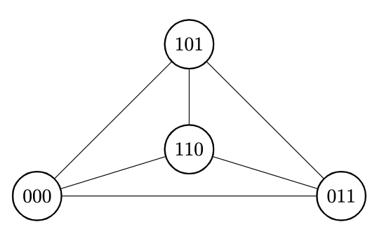
Example
For , the codewords form a tetrahedron, this the weight enumerator of that dual code is
and using the inverse relation, we find that the weight distribution of the original Hamming code is:

3.7 - Performance of Hamming Codes
There are many axes of measurements for the error detecting and correcting capabilities of codes at the output of the channel decoder:
: probability of decoder error or word error rate - the probability that the codeword at the output of the decoder is not equal to the codeword at the input encoder
: probability of bit error or bit error rate - the probability that the decoded message bits (extracted from a decoded codeword of a binary code) are no the same as the encoded message bits
: probability of undetected codeword error
: probability of detected codeword error - one or more errors detected
: probability of undetected bit error rate - the probability that a decoded message bit is in error and is contained within a codeword corrupted by an undetected error
: probability of detected bit error rate - probability that a received message bit is in error and contained within a codeword corrupted by a detected error
: probability of decoder failute - the probability that the decoder is unable to decode the received vector but able to determine that it is unable to decode
3.7.1 - Error Detection Performance
All errors of weight up to can be detected, so for computing the above probabilities, we consider patterns of weight and above.
If a codeword of a linear code is transmitted and error pattern happens to be a codeword, , then the received vector is also a codeword, hence the error pattern would be undetected. Thus the probability of undetected error is the probability that the error itself is a codeword.
to quantify this possibility, we consider only errors in transmission of binary codes over a BSC with a crossover possibility . The probability of any particular pattern of errors in a codeword is . Recalling that is the number of codewords in a code of weight , the probability that errors forms a codeword is , and the probability of undetectable error in a codewrod is then
The probability of a detected codeword is the probability that one more error occurs minus the probability that the error is undetected
Since these probabilities rely on knowledge of the weight distribution of the codes, which is not always available, it is common therefore to provide bounds on performance instead. For example, the upper bound on the probability of undetected error is the probability of occurrences of any patterns of weight meeting or exceeding . Since there are different ways that of positions can be changed, we have:
A bound on is simply
Example
For a code with , we have
If , then .
The correspondning bit error rates can be bounded as well. (Imagine being a naughty lil bit error rate uWu 🥵). can be lower bounded by the assumption that undetected codeword error corresponds to only a single message bit error, and upper bounded by the worst possible case that undetected codeword error corresponds to all message bits being in error:
3.7.2 - Error Correction Performance
Recall that an error pattern is correctable if and only if it is a coset leader in the standard array for the code, thus the probability of correction is the probability that the error is a coset leader. Let denote the number of coset leaders of weight . The set is then the coset leader weight distribtuion. Over a BSC with crossover probability , the probability of errors forming one of the coset leaders is
and the probability of a decoding error is thus the probability that the error is not one of the coset leaders:
which applies to any linear code with a complete decoder.
For a binary code with weight distribution , the probability of decoding error for a bounded distribution decoder is
The probability of decoder error can be bounded by the probability of _any_error patterns of weight greater than :
3.9 - Modifications to Linear Codes
An code is extended by adding an additional redundant coordinate, producing an code.
Example
The parity check matrix for a hamming code is extended with an additional row of check bits that check the parity of all the bits
The last row is the overall check bit row, and we can put the whole matrix into systematic form via linear operations yielding:
conversely, a code is punctured by deleting one of its parity symbols such that on code becomes an code.
Puncturing an extended code may return it to the original code (if the extension symbols are the ones being punctured). Puncturing can reduce to the weight of each codeword by its weight in the punctured positions. The of a code is reduced by punctring if the minimum weight codeword is punctured in a non-zero position. Puncturing an code times can result in a code with as small as .
A code is expurgated by deleting some of its codewords. It is possible to expurgate a linear code in such a way that it remains a linear code, but them inimum distance may increase. For example, deleting all odd-weight codewords
A code is augmented by adding new codewords. Addition of new codewordss may make a code non-linear, but the may decrease as well.
A code is shortened by deleting a message symbol, meaning a row is removed from the generator matrix (corresponding to the removed symbol), and a column is also removed, corresponding to the encoded message symbol such that an code becomes an code.
Finally, a code is lengthened by adding a message symbol, meaning a row and column are added to the generator matrix such that an code becomes an code.


4 | Cyclic Codes, Rings, and Polynomials
4.1 - Introduction
In which we introduce methods for deisgning generator matrices which have specific characteristics like minimum distance, and also reducing the prohibitive aspects of long codes and their corresponding standard arrays.
Cyclic codes rely on polynomial operations which allow use to incorporate design specifications. These operations leverage the algebraic structure known as a ring.
4.2 - Basic Definitions
Given a vector , the vector
is said to be the cyclic shift of to thr right. A right shift by produces
An block code is said to be cyclic if it is linear and if, for each , its right cyclic shift shift is also in .
Shifting operations can be convenienctly represented using polynomials. For example, the code can be represented by the polynomial:
The Division Algorithm
Let be a polymnomial of degree and be a polynomial of degree :
The division algorithm for polynomials assets that there exist polynomials (q for quotient) and (r for remainder) where and . The algorithm itself consists of polynomial long division. We say that is equivalent to :
If , then divides : , else .
A non-cyclic shift is represented by polynomial multiplication: . for a cyclic shift, we move the coefficient of to the constant coefficient position by taking this product modulo . Dividing by using the above "algorithm" we get:
s.t. the remainder upon dividing by is
4.3 - Rings
Rings exceed the usefulness of groups which are limited to their single operation; rings have two (count em) operations! A ring is a set with two binary operations addition, and multiplication, defined on s.t.:
- is an Abelian (commutative) group with the additive identity as 0.
- The multiplicative operation is associative
- Left and Right laws of distributivity hold:
- A ring is said to be commutative if
- Like groups, the collective ring may be referred to as just the representative set
- A ring with identity has a multiplication like identity on , typically defined .
Note, however, that the multiplicative operation need not form a group, as there may not be a multiplicative inverse in a ring, even if it has an identity. Some elements over a ring may have a multiplicative inverse, such elements are said to be units.
Example
- The set of matrices under usual definitions of addition and multiplication form a ring, though not commutative nor with comprehensive inverses as elements
- forms a rung, but not a group
Let be a ring and . For an integer , let denote with arguments. If a positive integer exists s.t. , then the smallest such positive integer is the characteristic of the ring . If no such positive integer exists, then is said to be a ring of characteristic .
Example
In the ring , the characteristic is 6. In the ring , the characteristic is . In the ring , the characteristic is 0.
4.3.1 Rings of Polynomials
Let be a ring. A polynomial of degree with coefficients in is
where . The symbol is said to be an indeterminate.
The set of all polynomials with an indeterminate with coefficients in a ring , using the usual operations for polynomial additions and multiplications, forms a ring called the polynomial ring: .
Example
Let and let , then some elements in are: with example operations:
Example
is the ring of polynomials with coefficients that are either 0 or 1 with operations modeulo 2. An example of arithmetic in this ring is:
since in this ring.
It is clear that polynomial multiplication does not have an inverse in general, e.g., in the ring of polynomials with coefficients , there is no polynomial solution to
Polynomials can represent a sequence of numbers in a single object. One reason polynomials are of interest is that their multiplication is equivalent to convolution of the sequence with
via the following polynomials:
and multiplying them: s.t. the coefficients of are
are equal to the values obtained by convolving .
4.4 - Quotient Rings
Returning to the idea of factor groups: given a group and a subgroup, a set of cosets is formed by "translating" the subgroup. We perform a similar construction over a ring of polynomials, assuming the underlying ring is commutative.
Consider the ring of polynomials (polynomials with binary coefficients) and the polynomial . In a ring of characteristic 2, . However, in other rhings, the poly should be of the form only. We divide polynomials up into equivalence classes depending on their remainder modulo .
E.g., the polynomials in all have remainder zero when divided by , so we write as the set generated by . The polynomials in all have remainder 1 when divided by , so we write it and so on:
Thus form the coset of modulo the subgroup which exhausts all possible remainders after dividing by . So every polynomial in falls into one of these sets.
We can define induced ring operations for both addition and multiplication which give some large tables similar to those we've seen for other groups modulo their order.
Let with such an addition table s.t. form an Abelian group with as the identity. However, not every element has a multiplicative inverse, so even does not form a group, but does form a ring denoted , the ring of polynomials in modulo . The general denotion of a ring be , and be .
Each equivalence class can be identified by its element of lowest degree:
Let be the set of these elements of lowest degree with addition and multiplication defined on polynomials modulo , the forms a ring.
Two rings are isomorphic if there exists a bijective function function called the isomorphism such that
Similarly, a ring is homomorphic if there exists a function that need not be a complete bijection preserving the above structural behavior.