Digest: Modeling Uncertainty
- Published on
- ∘ 18 min read ∘ ––– views
Tags
Previous Article
Preface
This post contains my notes of Daniel's presentation on Modeling Uncertainty with Monte Carlo simulations.
My copy of the spreadsheet containing the simulations can be found here.
Before and during the Manhattan Project, the legendary Italian physicist Enrico Fermi invented and used a variety of probabilistic techniques to study essentially deterministic questions which were too difficult for deterministic methods. Later when the MANIAC I computer was installed at Los Alamos, the usefulness of these methods exploded (no pun intended) and one colleague suggested that they be called Monte Carlo methods after another colleague's gambling uncle's patronage of the famous casino. So now, it's the umbrella term for algorithms that gamble with accuracy in order to blow past intractability barriers using computers.
If you have something that you want to workout but you can't do it analytically with math, either because that math hasn't been discovered yet, or you're just not good at math - don't panic! You have a computer which might be able to work it out by throwing 10 million darts at an oddly-shaped dartboard.
Quick Review of Probability Distributions
A probability distribution can be intuitively represented as a finite chunk of play-doh. The whole mass of the play-doh is the total distribution of all outcomes.
Suppose we have an uncertain outcome, like the result of the 2020 presidential race 1 week after the election. Based off of the most accurate polling results from that time, we might have a distribution that looks something like this:
| Candidate | % |
|---|---|
| Biden | 94 |
| Trump | 5 |
| Harris | 1 |
If you think these are the mutually exclusive possibilities, with any level of plausibility at all, then your job as a seeker of the truth is to distribute your probability distribution (play-doh) proportional to your confidence about the likelihood of each outcome. Crucially, you can never get more play-doh (the sum of all outcomes is capped at 100%: something has to happen, right?).
If for some reason, a 4th option looks at all possible and we want to assign some probability to it, we have to take the proportionate mass of probability play-doh away from one of the existing options. Similarly, if one of the options starts to look more likely we have to believe that the other options become less likely on penalty of incoherence.
Example 1: Rolling a Dice
Uncertainty and randomness are very similar. We can model our uncertainty about a single roll of a 6-sided die (1d6). We would uniformly distribute our confidence in across any of the 6 outcomes. A roll of a one should be assigned exactly 1/6th of our "play-doh", a roll of a two 1/6th, etc. (weighted dice not withstanding).
We can sample from our distribution by asking it for a randomly chosen number proportional the the probability mass we've assigned to that outcome. If we were to sample from our confidence in election outcomes, we should expect that 94% of the time, we would receive the outcome "Joe Biden", and if we were to sample our distribution of a fair roll of a dice, we should expect the outcome "five" almost 17% of the time and a roll of a "seven" 0% of the time.
Consider a more practical example: You're playing Dungeons & Dragons (a game whose mechanics are modeled around the results of various n-sided dice) with your buddies and stumble across an encampment of nasty orcs in boot cut jeans. In the inevitably ensuing violent encounter, you roll 1d20 to attack an orc and the outcome is a 20! Huzzah a critical hit. This means that you have the opportunity to double the damage that is output by your weapon. Suppose your weapon of choice is a gilded saber that deals 4d6 slashing damage. The rules of D&D 5e dictate that on critical hits, players are allowed to roll all of their damage dice twice and take the same of both sets of rolls (8d6 effective). However, some house rules also allow for simply doubling the damage of one set of damage rolls (4d6 * 2).
So the question is this: does it benefit you as the player to roll your damage dice twice, or simply double the result of a single damage roll. Using a trivial Monte Carlo technique and a spreadsheet, we can model the this situation and simulate thousands of dice rolls to analyze which outcome results in the highest damage:

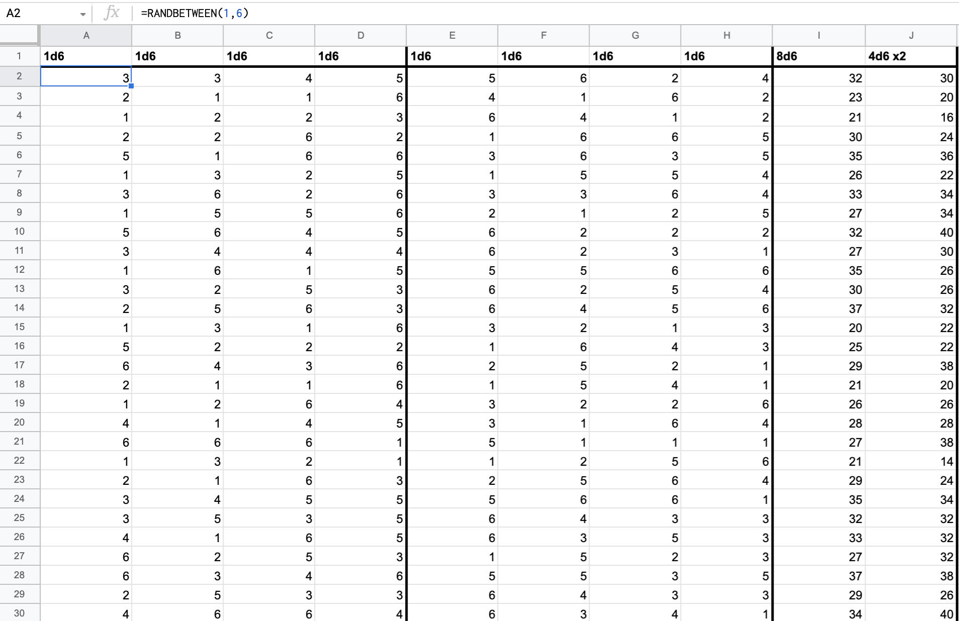
Here we have three sets of columns, the first two representing a set of 4d6 rolls (via the =RANDBETWEEN(1,6) function), and the third column showing us the output of taking 8d6 versus 4d6 * 2. By copying the formulae down to the bottom of the spreadsheet and pressing the Backspace key in any empty cell, we can recompute the random value of the rolls to our hearts content. We can also make quantitative observations about the distributions of the the results in the third section of columns (I,J). Of particular interest are:
- mean:
AVERAGE(I:I) - standard deviation:
STDEV(I:I) - minimum:
MIN(I:I) - maximum:
MAX(I:I)
Additionally, we can also directly compare the difference between two methods of calculating damage as well as plot the distributions of each:

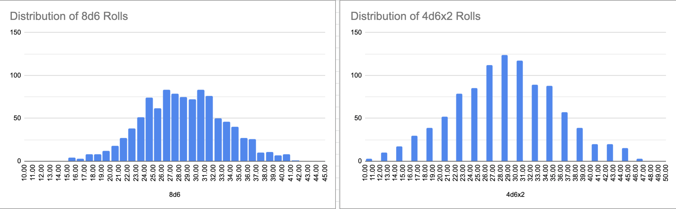
We can see that that the distributions are very similar, however, if we examine the minimums, maximums, and standard deviations we can see that
- on average, the minimum of 4d6 * 2 is less than the minimum of 8d6
- on average, the maximum of 4d6 * 2 is greater than the maximum of 8d6
- on average, the standard deviation –or "spread"– of 4d6 * 2 is greater than that of 8d6
| 8d6 | 4d6 *2 | |
|---|---|---|
| mean | 28.01201201 | 28.12212212 |
| std | 4.765214622 | 6.882138386 |
| min | 15 | 10 |
| max | 41 | 46 |
So, although the averages are nearly the same, 4d6 * 2 allows for more extreme values on either end of the range. That distinction would be very easy to miss without the full picture of our outcome distribution. That being said, over the course of your campaign against the orcs of the Hollow Earth, it makes almost nno difference which method of calculating your damage rolls you use, but the use of Monte Carlo Simulations allows us to tackle the seemingly opaque problem.
Example 2: Risk Management
It may surprise you to hear that it is equally valid to use these kinds of simulations for cases where there is no randomness involved: only your own uncertainty. The math of probability for random events corresponds exactly and uniquely to an extension of true/false logic where you have uncertainty, but no randomness at all. That correspondence means that we can work backwards and get answers to uncertainty questions by pretending that we can re-run the course of universal events numerous times. This correspondence between uncertainty on the one hand and randomness on the other is as deep and profound as they come.
So here's a risk management example with no randomness, just uncertainty, and it comes from the book How to Measure Anything - you should check it out. Suppose you are a manufacturer considering leasing a machine for part of your production process. You produce units! It costs $400,000/year paid annually with no early-cancellation. It's fancy and new fangled though, and you expect that it might save you money overall. Maybe. Probably. You have your internal experts put a 90% Confidence Interval on some important metrics: maintenance savings from having the machine, labor savings, raw materials savings, and production level. That is, your experts are coming up with a range for which they believe the true value to lie within with 90% certainty.
Calibration
Aside: 95% of humans are capable of accurate calibration, meaning that you can be trained in an afternoon to produce an accurate probability estimate in the sense that if you say something is 90% likely, it happens about 90% of the time. This is mostly a matter of learning what "90%" feels like or what "60%" feels like intuitively, as well as some tricks for avoiding common human biases that screw up numerical estimation.
Let's assume our experts have already been calibrated, so their Confidence Intervals really are 90% likely to contain the true values.
Spreadsheet time: let's plug in the (arbitrary) values that our experts have given us for the desired metrics:
| Metric | Value |
|---|---|
| MS 90% CI Lo | 10 |
| MS 90% CI Hi | 20 |
| LS 90% CI Lo | -2 |
| LS 90% CI Hi | 8 |
| RMS 90% CI Lo | 3 |
| RMS 90% CI Hi | 9 |
| PL 90% CI Lo | 15000 |
| PL 90% CI Hi | 35000 |
| Lease | 400000 |
| Total Annual Savings | 200000 |
Here, our rough estimate of total annual savings (if we do acquire the machine) are simply calculated by taking the sum of the midpoints of each savings Confidence Interval times the midpoint of Production Level minus the cost of the lease for the machine:
However, that outcome is only valid if each of those variables are equal to the midpoint's of their ranges: there's some uncertainty! We'd much rather know probabilities of breaking even or not. We can get that! But first, we need those ranges, with a shape. For example, sampling from the estimate range of Production Level that we got from our experts: is it equally likely to be the midpoint value vs. any other value in the Confidence Interval? If it was, that would be a Uniform distribution. Or, is there a central value which is more likely than those at the ends of the range – AKA a Normal or Gaussian distribution. Those are just two possibilities for the shape, but there are many other valid distribution shapes, each with their own purpose. You can reason out what the shape is, or we can just wave our hands and ask our experts (later on we could validate the accuracy of our chosen shapes as well), but for now it's safe to assume that all four of our distributions are normally distributed around the midpoints.
Fitting A Probability Distribution
"Fitting" here means that taking the parameters we need for some distribution, and hooking it up to our ranges. For any normal distribution, those parameters are just , and , the mean and standard deviation of those distributions, respectively. We have the mean of each distribution already, we've chosen it to be the midpoint, and we can get the standard deviation from the definition of a 90% Confidence Interval: we're 90% confident that the true value falls within that interval. Or in other words, 90% of the probability mass is distributed between those two endpoints of the range. So, we just need to convert the 90% confidence range into standard deviations.
Because who the heck has any intuition for what a standard deviation is, it is worth memorizing the fact that, for every normal distribution, 90% of the probability mass lies within the center 3.29 standard deviations. We can use this fact to re-scale our distributions into standard deviations just like we might perform any other unit conversion, say from miles to kilometers. We simply apply the fact that there are 3.29 standard deviations per 90% confidence interval:
And, using these parameters, we can just plug them right into our spreadsheet's =NORMINV(x, μ, σ) function to sample from a distribution of shape with a randomness factor of . Simple enough. So, let's do that for each of our estimated intervals like so:

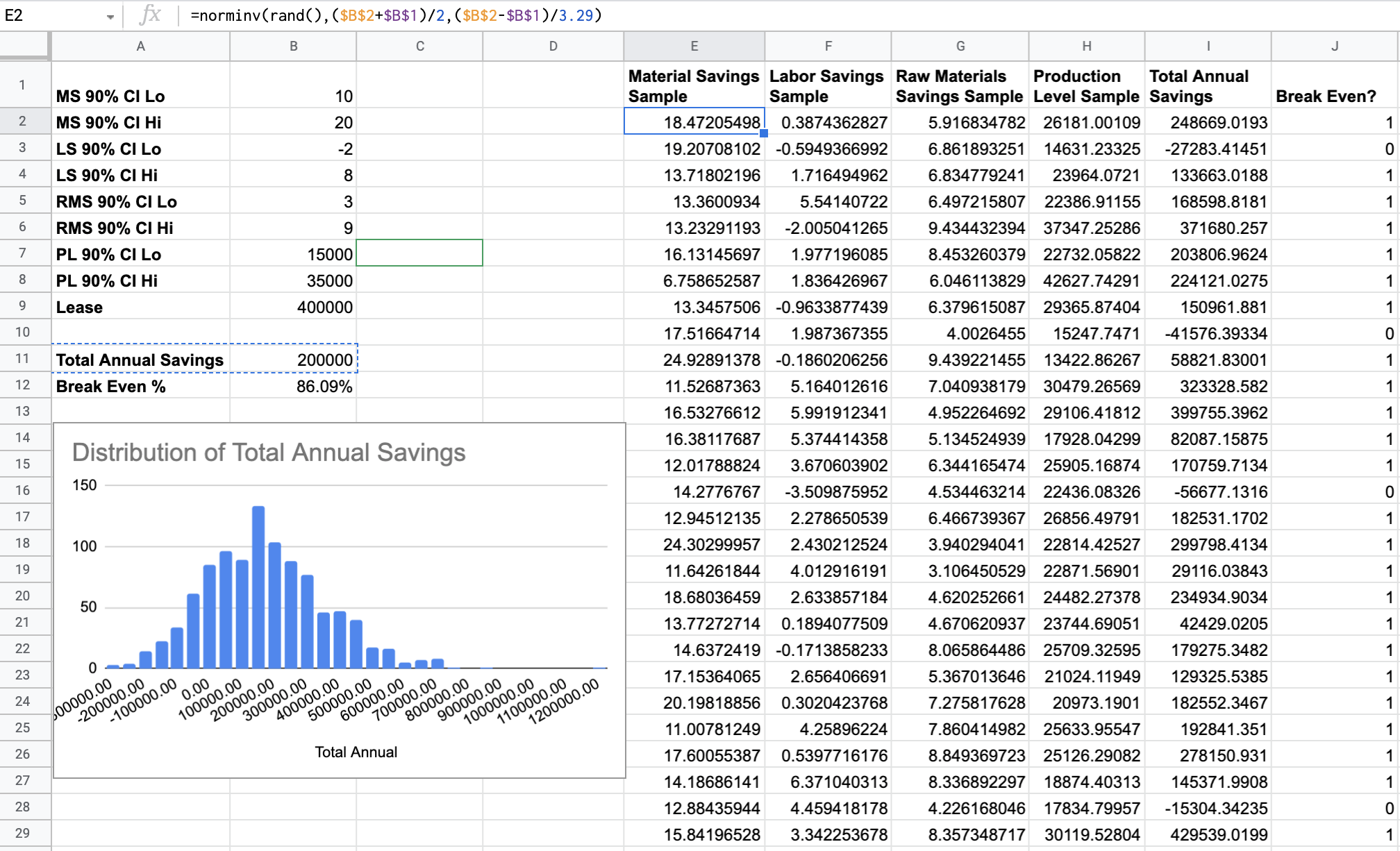
Columns I, J also give us additional information we will use to determine how likely it is that we break even for thousands of sampled value of each of our Confidence Intervals: turns out we break even around 86% of the time. Viewing our histogram we can visually confirm that number by seeing that the last negative number on the x-axis is rather to the left of the mean, making the vast majority of the probability mass imply that we're in the black.
And just like that we've solved our really complicated probability problem. We've modeled the real universe with this little toy universe, and then we sampled from our toy universe to get an answer which turns out to be comparable to the real one. This can vastly improve our ability to make informed decisions about the real universe.
So, how does the randomness sneak in? Nothing in the problem itself had any randomness, it's entirely deterministic. The deep correspondence between random sampling and uncertainty allowed us to take information we have about the shape of our uncertainty and model it using the shape of a probability distribution, and then we can sample that distribution thousands of times even though in the real world we cannot lease this machine a thousand times and re-run the universe with a single keystroke to see how it would go.
Other Types of Distributions we can Leverage
But it doesn't stop there, to quote the book this example is from:
"Our Monte Carlo simulation can be made as elaborate and realistic as we like. We can compute the benefits over several years, with uncertain growth rates in demand, losing or gaining individual customers, and the possibility of new technology destroying demand. We can even model the entire factory floor, simulating orders coming in, and jobs being assigned to machines. We can have inventory levels going up and down, and model work stoppages if we run out of something and we have to wait for the next delivery. We can model how the flow would change or stop if one machine broke down and jobs had to be reassigned or delayed."
That sounds fantastical and hard, but let's augment our model to go one step further. Say we're still wondering whether we need to lease this machine, but there's a major account that we might lose. Specifically, there's a 10% chance that Widgets R Us might decide to take their business elsewhere some month this year. Then, our production levels would decrease by 1,000 units/month after that. This would be a sudden change that a normal distribution can't model. So, are we doomed...?
No, we just need two more columns in our spreadsheet!
A "did we lose the account" column which me model with a Bernoulli or binary distribution which will output 1 with 10% probability and 0 with 90% probability (we can model this with a simple
=IF(RAND() < 0.1, 1, 0)function)A "How many months were left when we lost the account that year" column to hold the sunk cost of retaining the expensive lease on the machine without sufficient demand to justify it
So now, our new production level needs to be dependent on on these two columns as well as the decrease in production by 1,000 units if/when the account is lost like so and we calculate the Annual Savings amount just like we did before:

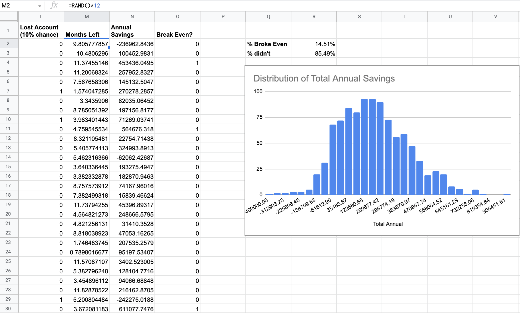
Turns out, this screws us really bad, and we break even less than 15% of the time. That's bad; turns out Widgets R Us is kind of important to our livelihood.
Conclusion
If the answer you get from the simulation has an unacceptable variance, i.e. turns out the number of possibilities will not break even or the spread is so large that, even though the mean looks okay, you're not super confident in the decision since if outcomes err towards the extremes, things could go terribly wrong, the model can tell you where you need to invest measurements to reduce uncertainty. Since every factor is itself represented by a probability distribution you can "ask about it's standard deviation" and see how confused you are correlated to how spread out the data is. You can then invest in some studies within your business to get those ranges tightened further than that 90% CI you started with.
Recall that 100% certainty is great! But almost always unattainable, therefore any reduction in uncertainty is valuable.
In summary, the "7 steps of a Monte Carlo simulation" are as follows:
The Equation - How would you compute the answer if there wasn't any uncertainty at all. If you just knew all of the variables, or at least all of the most important ones, how could you compute the answer you're looking for?
Calibrated Estimates - Get a calibrated estimate from somebody on the ranges of values each of those variables can take. Might as well always be a 90% confidence interval
To Model, or not To Model - At this point, you might be done. If you're 90% confident your values fall in those ranges, you can get the minimum and maximum values of the answer you care about, and it might already be acceptable for your purposes. Like with that machine example - if all you cared about was breaking even, and your minimum annual total savings was still positive, you'd be done
Model all Uncertain Variables - If you made it here, it means you care about the actual probability distribution of the answer, perhaps because you need the actual probabilities, or because you need to see if there are multiple peaks, or something else. So to go farther you need more than the confidence intervals, you need distribution shapes. Figure out which one makes the most sense for each variable, and fit it to your calibrated confidence intervals
Sample and Compute - Sample your component distributions, and plug the values into your equation. Re-run this simulation many many times. Thousands of times
Histogram - Each outcome is the result of a particular way the world may turn out to be. A histogram will tell you how the probability mass is distributed over the possible outcomes
Validate - You used several estimates and guessed at distributions in here, so it's prudent to collect some data from the real world to see if the distribution of the real data seems to match the statistics generated by the model. If so, you're likely good to move ahead with using your model for IRL predictions. If not, you likely made a mistake or left out important factors. This serves as a good check of the accuracy of your model
Monte Carlo Simulations in the Wild
Lastly, let's take a look at a practical example of these types of simulations: real election forecasting. FiveThirtyEight has a really fascinating page about how they arrive at their results which should make more sense with the background knowledge of how these types of simulations work.
Hopefully, it seems far less untenable how the organization go look up hundreds and thousands of factors which measure uncertainty about any (and every) given electoral district and compile a massive model of these underlying distribution models to arrive at their predictions for things like this election forecasting page, as well as March Madness, and everything else they do.
If you haven't seen enough, here's another interesting example which comes from Eli Dourado's election map on the night of November 8th:

This map is not based on any primary sources such as polls, voting trends, economic conditions etc. Instead, Eli used the free API for Betfair.com, which is a prediction market that functions exactly like a gambling site for horse races (partially because it is a gambling site for horse races). Contracts are priced by their odds and the odds constantly fluctuate in response to bets, they also correspond directly to probabilities. In a sense, Dourado leveraged the well-studied wisdom of crowds in the form of tens of thousands of people confidence intervals about the uncertain outcome of the 2020 presidential election.
Those two globs on the bottom are the probability distributions over the number of electoral votes cast for either party. People were offering each other rather conservative odds at that point as it was still election night, but you can see that most people still thought Biden would win as reflected by the peak of the blue hump aligning with ~310 votes on the x-axis and the red hump's peak (or mean) being closer to 230.
Two days later, those two humps were much much thinner and fifty times higher as the confidence –as reflected by the odds offered on Betfair– had honed in on the accurate results as people adjusted their contracts in light of new information (states being called for one candidate or the other).