Voyager 2
- Published on
- ∘ 60 min read ∘ ––– views
Previous Article
Next Article
Less morose and more present. Dwell on my gifts for a second
A moment one solar flare would consume, so why not
Spin this flammable paper on the film that's my life

Introduction
The date is July 9th, 1979. You are the Voyager 2 space craft, and for the past 23 months, you have been voyaging towards the outer planets of Earth's solar system. Cape Canaveral is over 440 million miles away and growing about half a million miles1 more distant every "day," but mankind has never been closer to Europa. Europa looks dope btw.
As with your twin craft on an exploratory mission of the same name, you are outfitted with numerous instruments for measuring the phenomena of the furthest reaches of our planetary system, including magnetic fields, low energy charged particles, cosmic rays, plasma, and plasmatic waves. You're also equipped with several cameras for capturing images of celestial bodies:

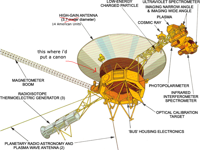
– Oh, and a Golden Record containing, amongst other things, a playlist curated by Carl Sagan himself. The images you capture will remain unparalleled in quality until the launch of the Hubble telescope, which won't happen for another decade. You are the king of space exploration.
However, considering the technological constraints of your mission's birth in 1972, your brain is reaaally small. So small that you can barely remember the first sentence of this exposition. Perhaps that's an exaggeration, but you're only working with about 70kb of memory which isn't even enough to store a novel. It's no help that despite the success of your predecessors, like the Apollo 11 mission, Tricky Dicky has cut funding to your program.
NASA's Response to Richard Nixon Slashing Funding
All this to say that you're firing on all cylinders, transmitting observed measurements and images in real time, as you encounter them, lest you forget.
Telemtry takes place via a 3.7 meter 14 foot high-gain antenna (HGA), which can send and receive data at a smooth 160 bits/second. Transmission is pretty much all-or-nothing, though, since your memory-span is as competitive as triceratops' or another maastrichtian creature of comparable synaptic ELO. There's no retry protocol, you've already forgotten your name, and you're hurtling through space faster than any prior man made object. No takesies backsies. No do-overs. And certainly no exponential backoff.
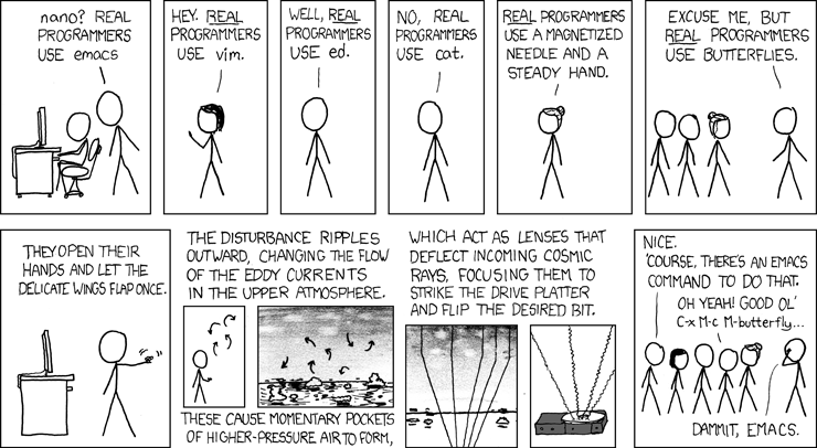
Among the numerous tried and true scapegoats which software engineers so often leverage when their code inevitably malfunctions are 🔥 cosmic ray bit flips 🔥. "How could I, in my infinite wisdom, have produced illogical behavior within my program. Nay, 'twas the sun who hath smited mine server farm and flipped the bits just so." (The anthropomorphisation of inanimate objects isn't going away any time soon). And, of course, there's the obligatory relevant xkcd:
But in OUTER SPACE, where part of the goal of the mission is to measure cosmic rays, said cosmic rays are slightly more prevalent. Bit flips are bound to happen at some point during the ~16 hour transit from the HGA back to Houston. And the engineers at NASA knew this to be the case before sending their half-a-billion dollar reconnaisance babies out into the wild. How, then, is the integrity of the data preserved?
Information Theory: Forward Correction
Luckily, with their backs against the wall, and Nixon's cronies looking for a reason to scuff the entire program,2 NASA did not have to also invent the wheel of Error Correcting Codes. Much of the groundwork of this realm of Information Theory had already been laid by Claude Shannon, John Hamming, and other bright minds of Bell Research and Signal Corps Laboratories. I have a few other ever-growing posts on Information Theory which house the supporting research for this post in particular, which go into more depth about what error correcting codes are and how they work. But the relevant bits have been included here, since that's kind of like the whole purpose.
In order to ensure that the information being beamed across the galaxy didn't get nuked in transit like leftovers in a microwave, the signals were encoded with additional data which offered some guarantees about allowable rates of error and mechanisms for correcting those errors. They employed a Golay Encoding, an extension of a Hamming Code, which is perhaps the most famous of binary error correction mechanisms. To understand how they work, let's start with some definitions and terminology.
Definitions
Error Control Codes
Error Control Codes are comprised of error detection and error correction, where an error is any bit in a message sequence which differs from its intended position. For example, our message might be and an error in this message might manifest as a pesky bit flip in the 3rd position: .
Entropy
Error is intrinsically related to Entropy, which is a measure of average uncertainty about random variables.
- For a discrete random variable , the information conveyed by observing an outcome is bits.
- If , an outcome of 1 is certain, then observing yields bits of information.
- Conversely, observing in this case yields ; a total surprise at observing an impossible outcome
Noiseless Coding Theorem
Shannon's Noiseless Coding Theorem states that given independent and identically distributed random variables, each with entropy :
- can be compressed into bits with negligible loss
- or alternatively compressed into bits entailing certain loss
- Given a noisy communication channel, a message of bits output by a source coder (like our HGA), the theorem states that every such channel has a precisely defined real numbered capacity that quantifies the maximum rate of reliable communication
In other words, provided that the rate of transmission is less than the channel capacity , there exists a code such that the probability of error can be made arbitrarily small
Code
An error correcting code of length over a finite alphabet is a subset of .
- Elements of are codewords in
- The alphabet of is , and if , we say that is -ary (binary, ternary, etc.)
- The length of codewords in is called the block length of
- Associated with a code is also an encoding map which maps the message set , identified in some canonical way with to codewords in
- The code is then the image of the encoding map
Rate
Given a noisy channel with a capacity , if information is transmitted at rate (meaning message bits are transmitted in uses of the channel), then
- if , there exist coding schemes (encoding and decoding pairs) that guarantee negligible probability of miscommunication,
- whereas if , then –regardless of a coding scheme– the probability of an error at the receiver is bounded below some constant (which increases with , exponentially in )
The rate of a code can also be understood in terms of the amount of redundancy it introduces.
which is the amount of non-redundant information per bit in codewords of a code , not to be confused with capacity.
- The dimension of is given by
- A -ary code of dimension has codewords
Distance
The Hamming Distance between two strings of the same length over the alphabet is denoted and defined as the number of positions at which and differ:
The fractional or relative Hamming distance between is given by
The distance of an error correcting code is the measurement of error resilience quantified in terms of how many errors need to be introduced to confuse one codeword with another
- The minimum distance of a code denoted is the minimum Hamming distance between two distinct codewords of :
- For every pair of distinct codewords in , the Hamming distance is at least
- The relative distance of denoted is the normalized quantity where is the block length of . Thus, any two codewords of differ in at least a fraction of positions
- For example, the parity check code, which maps bits to bits by appending the parity of the message bits, is an example of a distance 2 code with rate
Hamming Weight
The Hamming Weight is the number of non-zero symbols in a string over alphabet
Hamming Ball
A Hamming Ball is given by the radius around a string given by the set
Properties of Codes
- has a minimum distance of
- can be used to correct all symbol errors
- can be used to detect all symbol errors
- can be used to correct all symbol erasures – that is, some symbols are erased and we can determine the locations of all erasures and fill them in using filled position and the redundancy code
An Aside About Galois Fields
A significant portion of the discussion surrounding error correcting codes takes place within the context of Fields which sound more imposing than they actually are.
A finite or Galois Field is a finite set on which addition, subtraction, multiplication, and division are defined and correspond to the same operations on rational and real numbers.
- A field is denoted as , where is a the order or size of the field given by the number of elements within
- A finite field of order exists if and only if is a prime power , where is prime and is a positive integer
- In a field of order , adding copies of any element always results in zero, meaning tat the characteristic of the field is
- All fields of order are isomorphic, so we can unambiguously refer to them as
- , then, is the field with the least number of elements and is said to be unique if the additive and multiplicative identities are denoted respectively
They should be pretty familiar for use in bitwise logic as these identities correspond to modulo 2 arithmetic and the boolean exclusive OR operation:
| 0 | 1 | |
|---|---|---|
| 0 | 0 | 1 |
| 1 | 1 | 0 |
| XOR | AND | ||||||||||||||||||
|---|---|---|---|---|---|---|---|---|---|---|---|---|---|---|---|---|---|---|---|
|
|
Other properties of binary fields
- Every element of satisfies
- Every element of satisfies
Error Correction and Detection: Naive Approaches
There are numerous trivial means of encoding information in an effort to preserve its integrity. Some are better than others.
Repetition Code
A repetition code, denoted where is odd is a code obtained by repeating the input of length -bits times in the output codeword. That is, the codeword representing the input 0 is a block of zeros and likewise for the codeword representing the input 1.
The code consists of the set of the two codewords:
If is our desired message, the corresponding codeword is then
The rate of such a code is abysmal.
Parity Check
A simple Parity-bit Check code uses an additional bit denoting the even or odd parity of a messages Hamming Weight which is appended to the message to serve as a mechanism for error detection (but not correction since it provides no means of determining the position of error).
- Such methods are inadequate for multi-bit errors of matching parity e.g., 2 bit flips might still pass a parity check, despite a corrupted message
| data | Hamming Weight | Code (even parity) | odd |
|---|---|---|---|
| 0 | |||
| 3 | |||
| 4 | |||
| 7 |
Application
- Suppose Alice wants to send a message
- She computes the parity of her message
- And appends it to her message:
- And transmits it to Bob
- Bob recieves with questionable integrity and computes the parity for himself:
and observes the expected even-parity result.
If, instead, the message were corrupted in transit such that
then Bob's parity check would detect the error:
and Bob would curse the skies for flipping his bits. This same process works under and odd-parity scheme as well, by checking the mod 2 sum of Hamming Weight of the message against 1 instead of 0.
Interleaving
Interleaving is a means of distributing burst errors over a message. A burst error is an error which affects a neighborhood of bits in a message sequence, rather than just a single position.
For example, if we have a message:
which is struck by a particularly beefy cosmic ray such that a range of positions are affected:
By arranging the message in a matrix, transposing it, then unwrapping the matrix back into a vector, an effect analogous to cryptographic diffusion is achieved:
thus distributing the error across the message, making it easier to recover the complete message (lots of "small" errors are preferable to one gaping hole in our data as we'll see shortly).
Error Correction and Detection: Better Approaches
Hamming Codes
Hamming Codes are the most prevalent of more sophisticated mechanisms for error correction and detection. A -ary code block of length and dimension is referred to as an code.
- If the code has distance , it may be expressed as and when the alphabet size is obvious or irrelevant, the subscript may be ommitted
The simplest Full Hamming Code is and can be represented geometrically as a cube where the two code words are opposite vertices:

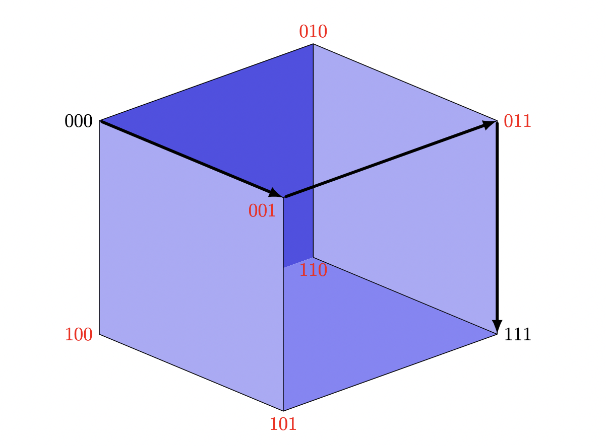
Opposite corners are necessarily three edges away from each other per this code's Hamming Ball property. We have two codewords which we assume are accurate (, ) representing our 1-bit message, and label all the other corners with "what we might get" if one of the bits gets corrupted.
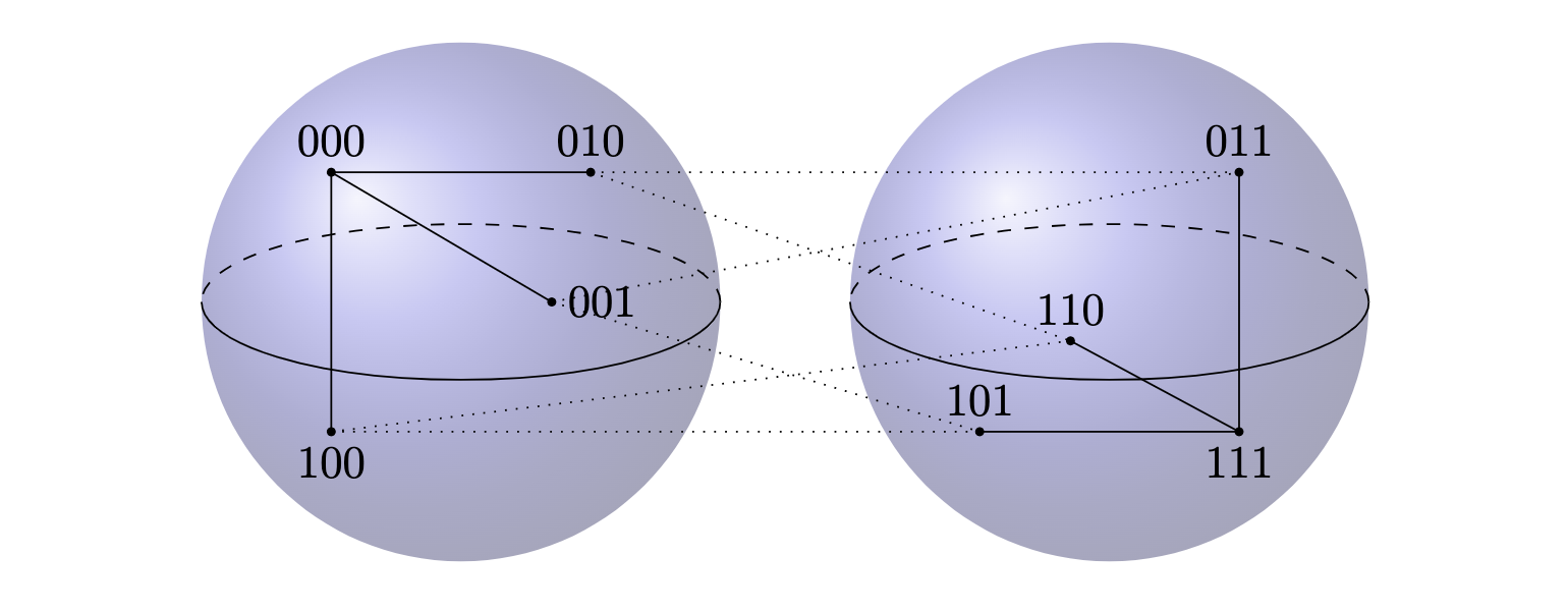
"But Peter," you might say, "that's not a sphere, that's a cube."
Go fuck yourself:

To decode, we take the correct message to correspond to the majority of the bits in our codeword. The corners adjacent to codeword are . If we "round" according to the majority of bits present, we preserve our target message of .
This code is "perfect" since each corner is used as either a target or a correction vector. If the receiver of an encoded message observes a correction vector, the decoding component will select the nearest composite codeword target.
The next full Hamming Codes are and , the former of which is also perfect on a 7-dimensional hypercube. Note that the degree of accuracy of all three of these codes are all , that is, one less than a power of 2.
Linear Codes and Generator Matrices
General codes may have no structure as we've seen above, but of particular interest to us are code with an additional structure called Linear Codes.
If is a field and is a subspace of then is said to be a Linear Code. As is a subspace, there exists a basis where is the dimension of the subspace. Any codeword can be expressed as the linear combination of these basis vecors. We can write these vectors in matrix form as the columns of an matrix which is called a Generator Matrix.
Hamming Codes can be understood by the structure of their corresponding parity-check matrices which allow us to generalize them to codes of larger lengths.
= is a Hamming Code using the Generator Matrix , and a parity matrix :
and we can see that , which means that if a message is encoded with yield and the product against the parity-check matrix is not 0, we know that we have an error, and we can not only deduce the location of the error, but also correct it.
Linear Construction
The original presentation of the Hamming code was offered by guess-who in 1949 to correct 1-bit errors using fewer redundant bits. Chunks of 4 information bits get mapped to ("encoded") a codeword of 7 bits as
which can be equivalently represented as a mapping from to (operations performed ) where is the column vector and is the matrix
Two distinct 4-bit vectors get mapped to the codewords which differ in the last 3 bits. This code can correct all single bit-flip errors since, for any 7-bit vector, there is at most one codeword which can be obtained by a single bit flip. For any which is not a codeword, there is always a codeword which can be obtained by a single bit flip.
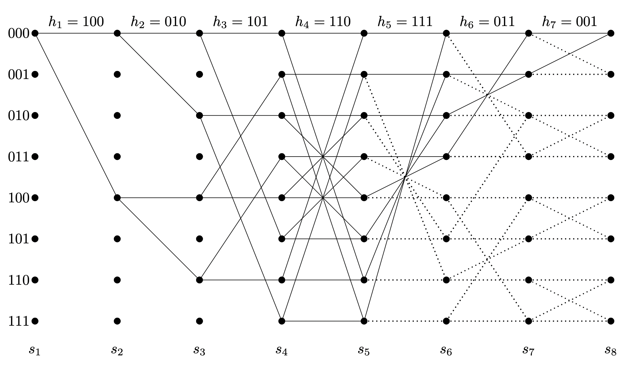
Graph Construction
A Wolf trellis for a Hamming Code is a graph associated with a block of a given called. Paths on the graph correspond to vectors that satisfy the parity check condition . The trellis states at the th stage are obtained by taking all possible binary linear combinations of the first columns of . The Viterbi Algorithm for decoding this representation finds the best path through the graph.
This is the Wolf trellis for the above Hamming Code:

Mogul
I'm just going to come out and say it. John Conway was a lizard man with an unparalleled case of chronic pattern-matching-brain. The man was of a different breed; the opposite of a maastrichtian.
Legend has it that a collegial IEEE Fellow of Conway's saw him dominating the schoolyard children in various games of Turning Turtles and Dots and Boxes and said "I bet you can't turn that into a Binary Lexicode of " to which Conway famously responded "Hold my beer."3
Attached for the author's amusement is an image of this absurd paper:

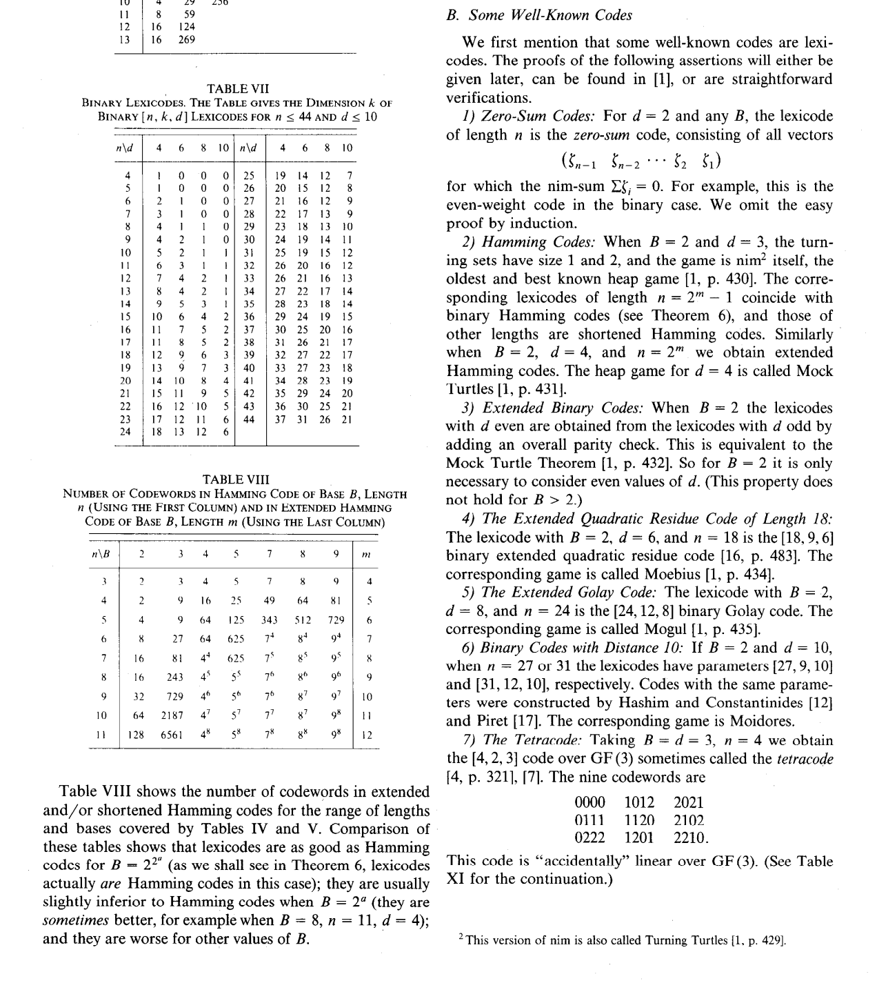
Madlad. Conway and Sloane showed that winning positions of a game of Mogal can be used to construct a Golay Code.
a position in Mogul is a row of 24 coins. Each turn consists of flipping from one to seven coins such that the leftmost of the flipped coins goes from head to tail. The losing positions are those with no legal move. If heads are interpreted as 1 and tails as 0 then moving to a codeword from the extended binary Golay code guarantees it will be possible to force a win.
Correcting Single Errors with Hamming codes
Suppose that is a corrupted version of some unknown codeword with a single error (bit flip). We know that by the distance property of , is uniquely determined by . We could determine by flipping each bit of and check if the resulting vector is in the null space of
- Recall that the nullspace of a matrix is the set of all -dimensional column vectors such that
However, a more efficient correction can be performed. We know that , where is the column vector of all zeros except for a single 1 in the th position. Note that the th column of which is the binary representation of , and thus this recovers the location of the error. We say that is the syndrome of .
Examples of Hamming Codes
- corresponds to the binary parity check code consisting of all vectors in of even Hamming Weight
- is a binary repetition code consisting of the two vectors
- is the linear Hamming Code discussed above
While fascinating, these codes can only correct 1 error, so a more robust code may be needed.
Perfect Codes
There are a few perfect binary codes:
- The Hamming Code
- The Golay Code
- The trivial codes consistng of just 1 codeword, or the whole space, or the repetition code for odd
The Golay Code
Like other Hamming Codes, the Golay Code can be constructed in a number of ways. A popular construction of consists of
when the polynomial is divisible by
in the ring . "The Ring" here is just a generalization of a Galois field with some additional properties. It is sufficient to think of it as a field with operations.
The seminal paper on this code was initially published by Marcel Golay in 1949 in an effort to devise a lossless binary coding scheme under a repetition constraint (i.e. all or nothing, no retries). It extends Claude Shannon's 7-block example to the case of any binary string. When encoding a message, the redundant symbols are determined in terms of the message symbols from the congruent relations:
In decoding, the 's are recalculated with the received symbols, and their ensemble forms a number on the base which determines unequivocally the transmitted symbol and its correction.
This approach can be generalized from via a matrix of rows and columns formed with the coefficients of the 's and 's in the expression above related times horizontally, while an st row added –consisting of zeroes, followed by as many ones up to ; an added column of zeroes with a one for the lowest term completes the matrix for .4
The coding scheme below for 23 binary symbols and a max of 3 transmission errors yields a power saving of db for vanishing probabilities of errors, and approaches 3 db for increasing 's of blocks of binary blocks, and decreasing probabilities of error, but loss is always encountered for .
Using Golay Codes
The Golay Code consists of 12 information bits and 11 parity bits, resulting in a Hamming distance of 7: .
Given a data stream, we partition our information into 12-bit chunks and encode each as a codeword using special Hamming Polynomials:
We'll define our data as a trivial message of convenient length 12:
We append 11 zero bits to the right of our data block:
and perform division on the polynomial via the bitwise XOR operation:
Thus, yields : the syndrome of the message. The 11-bit zero vector is replaced with the syndrome, and if decoded with a Hamming polynomial the resultant syndrome or remainder will be 0:
A 1-bit error in transmission such as
would have a syndrome of 1.
However, syndrome should not be construed as proportionate to magnitude of error. A 1-bit error in the information bits yields a syndrome of 7:
An algorithm for decoding the parity bits of a Golay Code is as follows:
- Compute the syndrome of the codeword. If it is 0, then no errors exist, and proceed to (5).
- If , the syndrome matches the error pattern bit-for-bit and can be used to XOR the errors out of the codeword. If possible, remove errors and toggle back the toggled bit and proceed to (5).
- Toggle a trial bit in the codeword to eliminate one bit error. Restore any previously toggled trial bit. Proceed to (4), else return to (2) with .
- Rotate the codeword cyclically left by 1 bit and go to (1)
- Rotate the codeword back to its initial position.
How to Actually Beam Them Up, Scotty?
"Okay but how do these encodings actually get transmitted? I mean we're talking about space here, not an IRC channel."
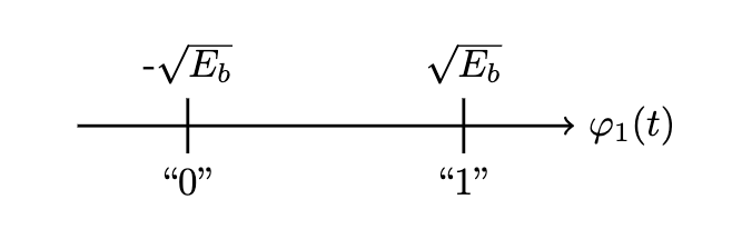
Binary Phase-Shift Keying is a technique for mapping a binary sequence to a waveform for transmission over a channel. Given a binary sequence , we map the set via
We also have , a mapping of a bit or () to a signal amplitude that multiplies a waveform which is a unit-energy signal:
over . is the amount of energy required to transmit a single bit across the channel. A bit arriving at can be represented as the signal where the energy required to transmit the bit is given by
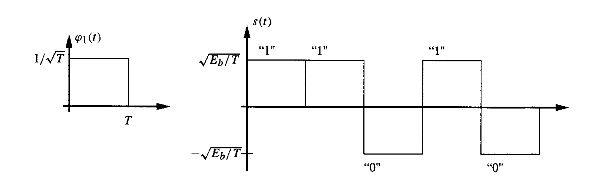
The transmitted signal are points in a (for our purposes: one-) dimensional signal space on the unit-energy axis

such that a sequence of bits can be expressed as a waveform6:

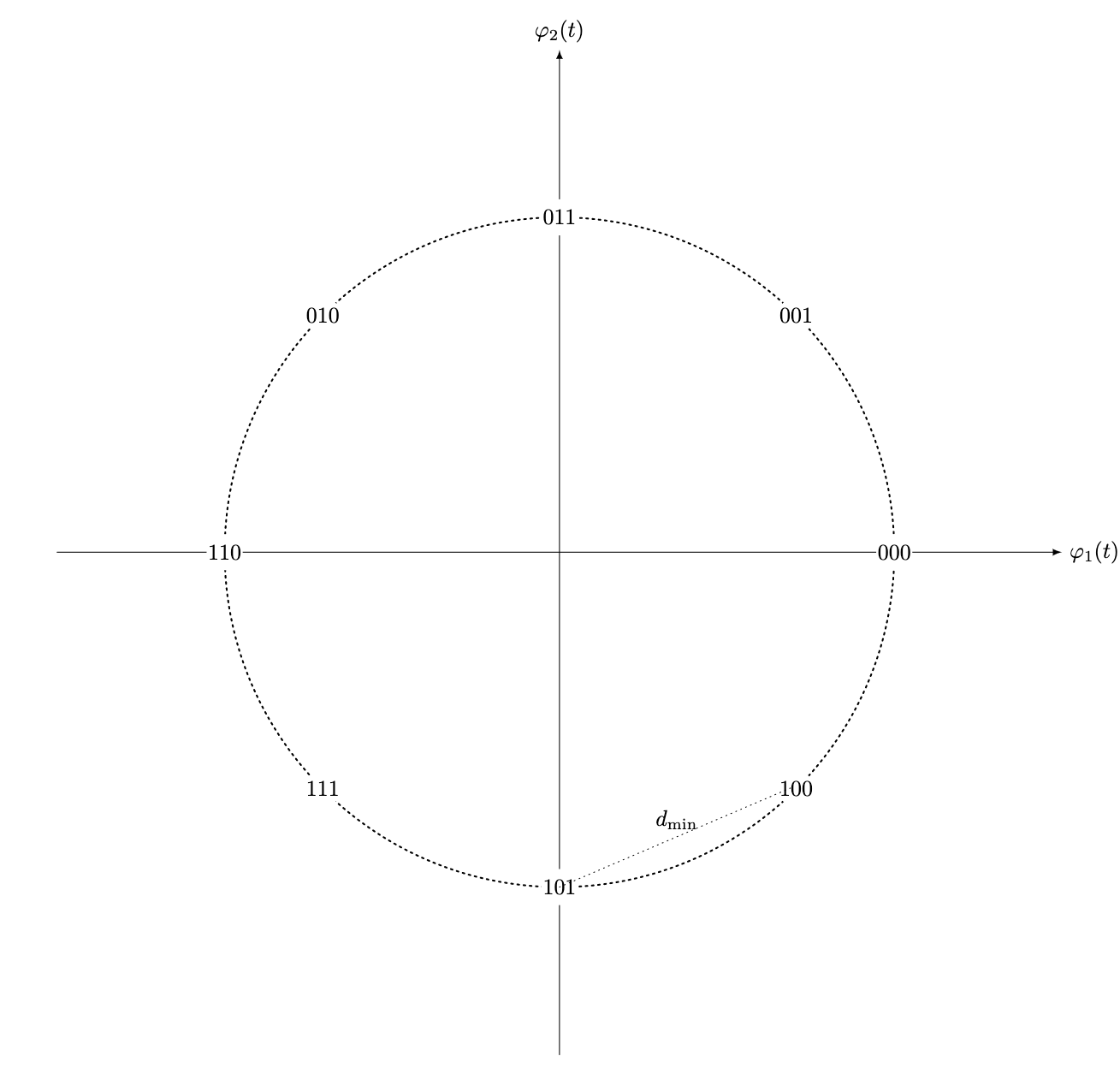
We can expand this representation to two dimensions by introducing another signal and modulating the two to establish a signal constellation. Let , be the number of points in a constellation. -ary transmission is obtained by placing points in this signal space and assigning each point a unique pattern of bits.

Once our message has been encoded for error correction, and further transformed via signal constellation into a waveform, it must be read by a receiver somewhere. We call the transmitted value , chosen with prior probability . The receiver uses the received point to determine what value to acsribe to the signal. This estimated decision is denoted
and is used to determine the likelihood of observing a signal given a received data point . The decision rule which minimizes the probability of error is to choose to be the value of which maximizes , where the possible values of are those in the signal constellation:
Since the denominator of this expression does not depend on , we can further simplify:
leaving us with the Maximum A Posteriori decision rule. And, in the case that all priors are equal (as we assume with our binary code), this can also be further simplified to a Maximum Likelihood decision rule:
.
Once the decision is made, the corresponding bits are determined by the constellation; the output of the receiver is a maximum likelihood estimate of the actual bits transmitted. is selected to be the closest point according to Euclidian distance .
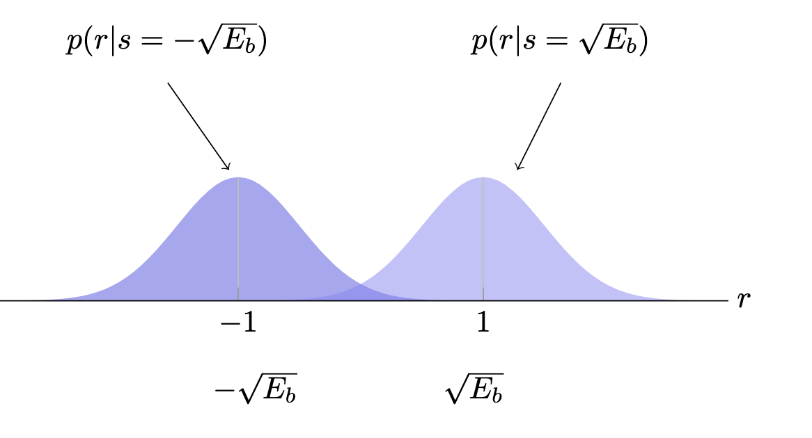
The "raw" signal distributions are dueling Gaussians about the corresponding mean measurements of under our projections to .

and the weighted conditional densities of the Maximum A Posteriori decision rule distribution resemble:
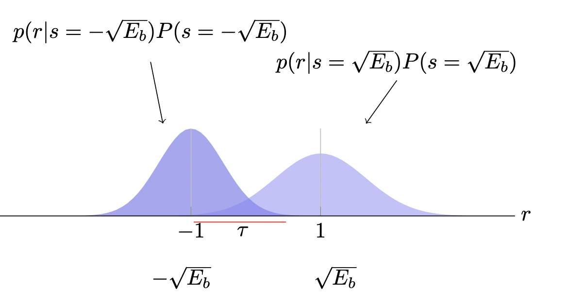
where is threshold at which
which, when met or exceeded, implies that our decision rule becomes
which can be computed explicitly by solving for the intersection point:
.
Binary Detection errors in signal reception can still occur when a received point exceeds this threshold which can be computed with a Cumulative Distribution Function:
which we will use in measuring the performance of various coding schemas.
In the special case where measured signal strengths are assumed to be equal, the overall probability of error is given by:
where are signals.
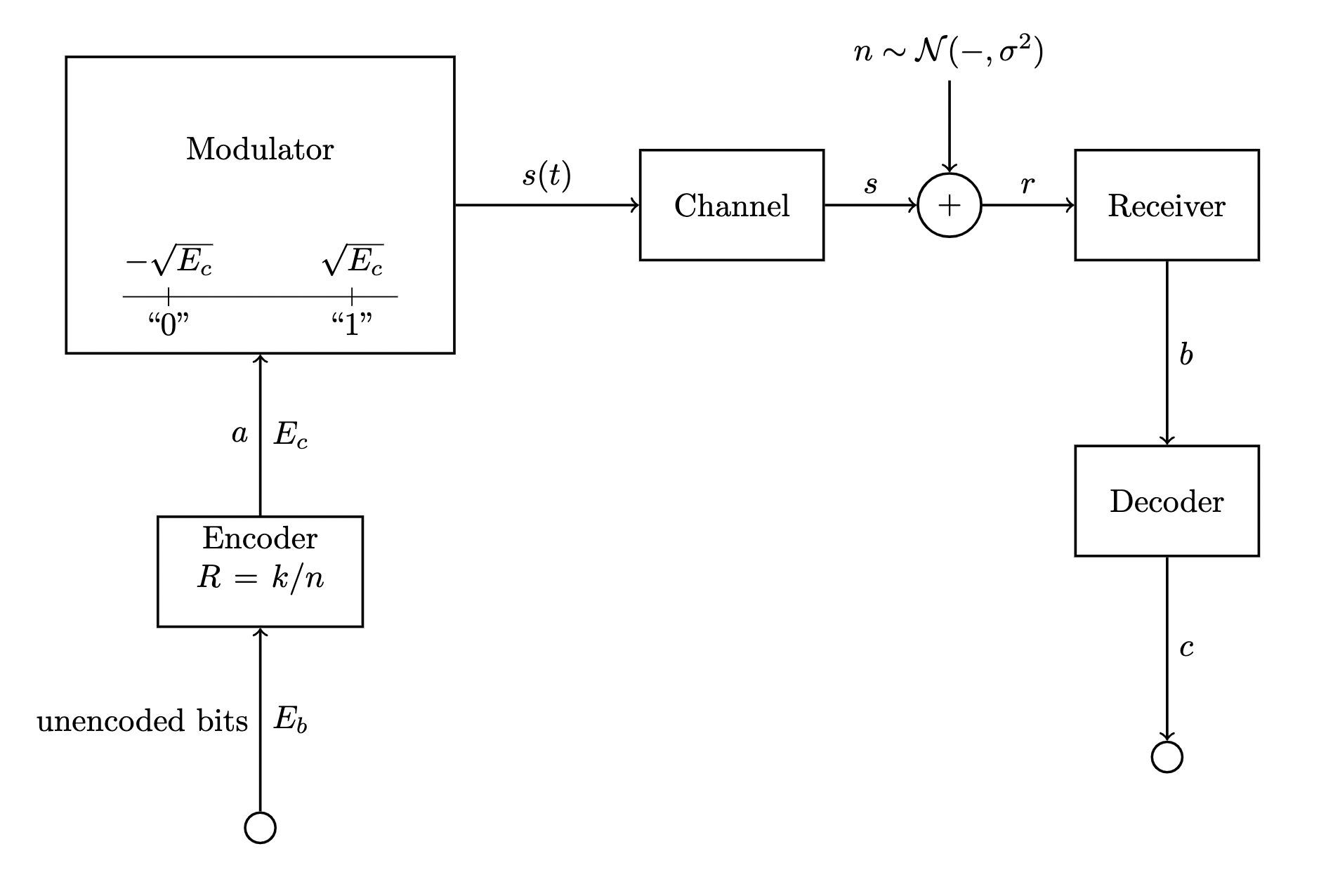
All together, our Binary Phase-Shift Keying transmission system from HGA to Houston looks something like this:

Performance of Error Correcting Codes
How "expensive" is it to add these redundant bits to our transmission? Is it worth it?
What, you didn't think Europa looked cool?
Recall that in our system, inputs result in output bits where . is the rate of our correcting code, and for some arbitrary transmission budget we have joules/bit for the unencoded bits of data which is spread over more encoded bits. This relationship can be expressed as , where is understood as the "energy per coded bit," and necessarily meaning that unencoded transmission performs better in terms of energy, but we risk error by omitting the encoding process.
At the receiver, the detected coded bits are passed to the decoder to attempt to correct errors. In order to be of any use to us, the value of the code must be strong enough so that the bits received can compensate for the lower energy per bit in the channel.
Reptition Code
For a repetition code with a transmission rate of 1 bit/second, we must send coded bits/second and with times as many bits to send, there is still a constant amount of power shared by all bits: . Thus there is less energy available for each bit to convey information, and the probability of error is
Notice that the probability of error is higher as a result of using such a code! 💩
Golay Code
As a concrete example, let's compare the relative performance of a Golay Code against a pure stream of data, that is a message that has 0 redundant bits (but high risk of data loss):
- System transmits data bits directly
- System trasmits a total of 23 bits for every 12 data bits
We assume a constant unit of power is available to each system. System employs a Golay Code transmitting roughly twice as many bits as , so the strength of energy across each bit is halved. is the amplitude of detected output, which will be since ,7 but the cost of these penalty bits is necessary to ensure corrective ability. is the measure of penalty in terms of error for decreasing the power of transmission by a factor of 2.
| 1 | |||
Thus, is twenty-times more susceptible to error because of the reduced strength of energy per bit, meaning that the receiver will have more difficulty correctly measuring which codeword is being transmitted. However, the redundancies which the Golay Code introduces allow for guaranteed recovery of the complete message, whereas one in two thousand bits in our pure stream of data from are simply lost forever like the Bitcoin I mined on the family computer ten years ago.
The Hadamard Code
The dual of the Hamming Code has a generator matrix which is a matrix whose rows are all non-zero bit vectors of length . This yields a code and is called a simplex code.
The Hadamard Code, is obtained by adding an all-zeros row to .
is a linear code whose generator matrix has all -bit vectors as its rows. Its encoding map encodes by a string in consisting of the dot product for every . The Hadamard code can also be defined over , by encoding a message in with its dot product with every other vector in that field.
It is the most redundant linear code in which no two codeword symbols are equal in every codeword, implying a robust distance property:
- The Hadamard Code has a minimum distance of .
- The -ary Hadamard Code of dimension has a distance
Binary codes cannot have a relative distance of more than , unless they only have a fixed number of codewords. Thus, the relative distance of Hadamard Codes is optimal, but their rate is necessarily poor.
Limits of Error Correcting Codes
The Hamming and Hadamard codes exhibit two extreme trade-offs between rate and distance
- Hamming Code's rates approach 1 (optimal), but their distance is only 3
- Conversely, Hadamard Code's have an optimal relative distance of , but their rate approaces 0
The natural question that follows is is there a class of codes which have good rate and good relative distance such that neither approach 0 for large block lengths? To answer this question, we consider asymptotic behavior of code families:
Define a code family to be an infinite collection , where is a -ary code of block length , with and
The Familial Rate and Distance of a category of codes are denoted:
A -ary family of codes is said to be asymptotically good if its rate and relative distance are bounded away from zero such that there exist constant
While a good deal is known about the existence or even explicit construction of good codes as well as their limitations, the best possible asymptotic trade-off between rate and relative distance for binary codes remains a fundamental open question which has seen little advance since the late 70s, in part due to the the fundamental trade off between large rate and large relative distance.
The Hamming and Hadamard Codes help to highlight the flexibility and main take aways of the Channel Coding Theorem as outlined by Wiley:
- As long as , arbitrarily reliable transmission is possible
- Code lengths may have to be long to achieve desired reliability. The closer is to , the larger we would expect to need to be in order to obtain some specified degree of performance
- The theorem is general, based on ensembles of random codes, and offers little insight into what the best code should be. We don't know how to design the, just that they exist
- Random codes have a higher probability of being good, so we can reliably just pick one at random
What then, is the problem? Why the need for decades of research into the field if random selection of a code might be our best bet?
The answer lies in the complexity of representing and decoding a "good" code. To represent a random code of length , there must be sufficient memory to store all associated codewords, which requires bits. To decode a received word , Maximum Likelihood Estimation decoding for a random signal requires that a received vector must be compared with all possible codewords. For a middling rate of , with block length (still relatively modest), comparisons must be made for each received signal vector... This is prohibitively expensive, beyond practical feasibility for even massively parallelized computing systems, let alone our 70kb, Fortran-backed integrated circuit.
Conclusion
Today Voyager 2 is 12 billion miles away, and traveling over 840,000 miles further each day. We're still actively transmitting and receiving data (intact) from both of the Voyager spacecrafts.
It's somewhat difficult to appreciate the absurd amounts of genius which made make that feat possible. I find the difference in the orders of magnitude between the 30,000-odd words worth of computing power available to the space craft and the billions of miles of distance separating the scientists from their experiment which they expertly designed to outlive them to be mind boggling.
Pretty sick if you ask me.
Happy Discovery of Adrastea day.
References and Footnotes
- Lexicographic Codes: Error-Correcting Codes from Game Theory
- Voyager timeline
- Other geometric representations of codes
Footnotes
Um, so yeah. I'm going to be using imperial measurements. If only there were a convenient way to quickly convert between metric and imperial, say the 42nd and 43rd numbers of the Fibonacci sequence? Easily, we recall that 433,494,437 precedes 701,408,733 in the sequence and thus, 440 million miles is roughly 700 million kilometers. ↩
Nixon was actually a large proponent of the space program, but this story needs an antagonist, and he's as good as any. ↩
More lizard brain pattern matching at work here. ↩
Marcel was a crackhead for thinking this is a sufficient explanation for the construction. The Paper, if it can even be called that, could fit on a napkin. Mathematicians of a certain flavor exhibit the same kind of stoney-Macgyver behavior, see Conway. ↩
These diagrams took me several hours. Please clap. ↩
This diagram was taken from Error Correction Coding: Mathematical Methods and Algorithms which is a good book. ↩
Energy in a wave is proportional to Amplitude squared. ↩