2.3728596
- Published on
- ∘ 81 min read ∘ ––– views
Previous Article
Next Article
Introduction
I ask the reader to call to mind some of the great rivalries over the centuries: Achilles vs. Hector, Tesla vs. Edison, Ford vs. Ferrari, ... and of course Vassilevska Williams vs. Le Gall.
In the past decade, a handful of researchers have been duking it out over matrix multiplication algorithm performance and it seems like no one is paying attention?!?! Today we're gonna poast about this paper "A Refined Laser Method and Faster Matrix Multiplication,"1 by Josh Alman and Virginia Vassilevska Williams which shatters, okay well ... it doesn't really shatter the previous best method – but it makes a notable improvement which can likely be generalized to other classes of tensors to push the upper bound even lower.
The Problem of Matrix Multiplication
Given matrices over some field , we want to compute s.t.
but we wanna go fast. How many operations over the field (addition, multiplication, division) are needed to compute ? The authors of this paper posit that there are tight bounds on the number of operations:
but if you've ever taken a linear algebra exam, we know that we can certainly do worse than cubic time to apply the standard inner-product algorithm, making several arithmetic mistakes along the way to compute the result matrix.

The Inner Product Algorithm
The first (and usually last method) most of us pedestrian matrix multipliers learn just takes the dot product of all the rows of the first matrix with the columns of the second matrix. This is fine, but slow, as it requires many multiplication operations which are more expensive than additions. I won't get into the weeds (perhaps my next muse...) since there's plenty of weeds at the current layer of abstraction, but suffice it to say that the additions become asymptotically irrelevant and multiplication at the ALU level typically requires several additions, whereas the inverse is not true.2
If we're just limited to pen and paper, and compelled to multiply two matrices and , the approach we'd probably use would look something like this:
which is multiplications. Meh.
History of the Problem
Coppersmith and Winograd are heavily cited as a "black box" for other computational performance benchmarks or building blocks in the field of computational theory since matrix multiplication is the foundation of pretty much all applied linear algebraic questions. Operators including matrix inversion, rank, determinant, lower-upper factorization/decomposition, eigen anything-ing, etc. Matrix multiplication also has applications in other fields such as graph theory, complexity theory, etc. so the motivation for wanting to go fast is well established.
Up until 1969, it was thought that it wasn't possible to compute the product of two matrices in faster-than-cubic time. In fact, the discovery of a faster method was made by Volker Strassen when trying to prove that standard Gaussian elimination (an approach) was optimal. This discovery was published in a paper aptly titled Gaussian elimination is not optimal.2 And this was a watershed moment for investigation into faster means of matrix multiplication using various methods:

Till the past decade or so, when only minor improvments on the order of hundredths of thousandths of operations are being shaved off. This might not seem like much, but for massive matrices like the ones you print out to help you on your final exam, these add up. Additionally, the academic heart strives to know the theoretic optimum. Ultimately, the question of Matrix Multiplication optimization boils down to one of asymptotic rank of a Matrix Multiplication Tensor.
The Matrix Multiplication Tensor
There are many representations or interpretations of what a tensor is:
- a multidimensional array:
- A bilinear map, taking two vectors to a third vector:
- A trilinear map, taking three vectors to a scalar:
- a multilinear polynomial:
The last interpretation is the one widely used in the Matrix Multiplication Problem since it's useful for encoding the notion of a "problem" within another problem.
We define a tensor as a multilinear polynomial over sets of formal variables so that
where are elements of some field e.g. . As mentioned before, every tensor under this interpretation (which is equivalent to any of the others) defines a computationl problem: for given vectors , and every (the number of polynomials we want to compute), we want to compute the coefficients of which is a bilinear polynomial:
The Matrix Multiplication Tensor (MMT), then, is the one to solve our problem. For , define:
to be the MMT for multiplying two matrices .
In general, the coefficient of in is the ()th entry of
The Matrix Multiplication Problem
The formal problem that we encode as an MMT is the Matrix Multiplication Problem:
about which we care for the asymptotic rank.
Tensor Rank
In general, is the complexity of a tensor, and a tensor is just the natural generalization of a matrix. The total of a tensor is the minimum number of one tensors whose product equals . We define a tensor of one if there exists such that our tensor can be expressed as the product of linear combinations:
We often express this tensor as (read " tensor tensor "). Matrix is the same just without the third dimension.
A mathematical object is just a scalar, an object is a vector; an matrix, and objects are tensors.
At a high level, the decomposition of into rank one terms provides an algorithm for multiplying arbitrary matrices using scalar multiplications.
Properties of Tensor Rank
- Lemma: if , then via the recursive application of implying . We can express this as the sum of terms that are linear combinations of the entries of our tensor times the linear combination of the entries ... and so on:
and we use this expression to develop an algorithm for constant-sized matrices e.g. representing two matrices, and we use it to recursively solve for the product of larger matrices whose entries are themselves matrices:
The algorithm is:
- For all recursively compute
- For coefficients of , compute
This algorithm can be used to multiply block matrices. Via recursive application, we can multiply matrices of arbitrary size, with the rank controlling the asymptotic complexity of the algorithm: a matrix can be multiplied with asymptotic complexity of .
Thus, is a "block" and a comparatively cheap quantity to compute since it's just a summation with few multiplications compared to our naive approach. Additionally, is cheap to compute since it's just another linear combination which can be computed in linear time. So, the whole runtime of this algorithm is dependent on the number of recursive calls to compute our blocks which is , hence why we are concerned with the asymptotic rank of the MMT, and also how Strassen got
Similarly, in 1978 Pan achieved via
It was around this time that people stopped analyzing fixed size Matrix Multiplication Problems because it quickly becomes unwieldy to work with such large objects. So, the method for analysis changed. In 1987, Coppersmith and Winograd published a new method for designing Matrix Multiplication Algorithms.4 These methods –which have become more or less standard as far as I can tell– rely on two components:
- an Algebraic Identity: corresponding to a representation of some small tensor
- a Method for Analyzing the Identity: which is the method of extracting a Matrix Multiplication Algorithm from other tensors
| Publication | Algebraic Identity | Analysis |
|---|---|---|
| Strassen, 1969 | MM using only 7 multiplications | Simple, recursive approach |
| Coppersmith, Winograd 1987 | The tensor and its powers | Laser Method, introduced by Coppersmith, Winograd, and Strassen |
| Stothers, 2010 | Laser Method | |
| Vassilevska Williams, 2011 | Laser Method | |
| Le Gall, 2014 | Laser Method | |
| Vassilevska Williams, 2020 | Refined Laser Method |
The Laser Method
The Laser Method is an indirect technique for extracting Matrix Multiplication Algorithms out of other objects. It was developed by Strassen, and optimized by Coppersmith and Winograd. Crucially, as recently as 2019,5 Josh Alman proved the correctness of the Laser Method, showing that for tensors for which it can be applied, if any other method could achieve the optimum of using , then so can the Laser Method. Therefore, the Laser Method is optimal for a certain subset of tensors.
How does it work?
The Laser Method is a composition of reduction problems:
- Take some algebraic problem that we have an efficient algorithm for
- Show how to reduce the problem of Matrix Multiplication to
This is nearly identical to Strassen's original approach to proving sub-cubic time. E.g. given the algebriac problem instance of Matrix Multiplication for two matrices:
evaluate the four polynomials:
Hell, we may as well throw them into the matrix box that they belong in:
and suppose we can solve some other problem , given terms
we want to compute the 5 polynomials:
At a high level, our goal is to embed matrix multiplication into this similar, and notably larger (by the introduction of the terms) problem . Our measure of success is removal of some inputs and outputs of to transform it into the Matrix Multiplication Problem:
which would leave us with just the polynomials needed for Matrix Multiplication as part of . But how can we cancel those inputs and outputs?
If we phrase in terms of a tensor that we have a known, good bound for such as the MMT:
we must now show how to reduce it to where:
The way we achieve this reduction is be setting some of the variable of our instance of to zero. Setting yields our desired Matrix Multiplication tensor exactly (which is not always the case as we'll see shortly):
This is called zeroing-out a tensor which is similar to the notion of reducibility in complexity theory. We denote that is reducible to via zeroing as "" which does have a well-defined bound.
Lemma: If , then , so
if , then .
Brief aside about the Strassen method
Strassen showed that it is possible to compute those polynomials using the following identities:
where
where
which reduces the number of matrix additions from 18 to 15, and the multiplications from 8 to 7!
Laser Method
The Laser Method is a bit more complicated than just the above reduction, namely due to the fact that it becomes increasingly challenging to zero out terms without removing terms we still need for the Matrix Multiplication proper for larger input matrices.
Thus, the Laser Method instead reduces direct sums of Matrix Multiplication Tensors to powers of tensors with a special structure via the zero-out reduction illustrated above. The process looks like this:
and composing all of these gives us a reduction from Matrix Multiplication to a tensor .
Direct Summation
For some tensor i.e. , we can add it with a slightly modified copy of itself yielding a "regular" sum:
Observe that both copies share a variable. Conversely, a direct sum of two copies of are completely disjoint: they have no variables in common despite summing over the same set of variables:
Schönhage showed that, because of this disjoint-ness, upper bounds for MMTs also yield upper bounds for via the following theorem:6
If the direct sum of copies of have m then .
This means that we just have to show that the rank of disjoint copies of some MMT is smaller than times the rank of the original tensor. This is the first step of the method diagrammed above:
Tensor Exponentiation
Now, for the other half of the method, what the hell does this mean: . We need to define what it means to exponentiate a tensor. First, we define the product of two tensors via the Kronecker Product.
For tensors over variable sets , respectively, where
not only does our notation converge on sanscrit, but we get a definition of a tensor product:
over , , and is given by:
which we immediately generalize into the definition of the power of a tensor:
Lemma: The product of any two MMTs can be combined into a product of their dimensions: which precisely corresponds to our idea of "blocking."
Observe that will contain tuples over each variable set of the original tensor, so we get larger and larger variable sets, but the rank is guaranteed to be bounded by the individual ranks of the tensors being multiplied per the following:
Lemma: , so
and sometimes, .
From these lemmas, we can get an expression for asymptotic rank:
For example, for the MMT, , but the rank of the th power of it is ! Thus, asymptotic rank is the secret workhorse of all modern Matrix Multiplication algorithms. This completes the right half of our methodology diagram:
We can interpret this to mean: if we have a bound on the asymptotic rank of the tensor, we also have a bound on the asymptotic rank of its th power. So now we just have to show the reduction via Laser Method allowing us to compose the left and right halves. If we can compose these steps for sufficiently large , then we can get a really good bound on .
Laser Method
Finally, the middle bit:
The Laser Method takes a tensor with a "special structure" and uses that structure to reduce the direct sum to for large functions of by zeroing out many variables of yielding huge disjoint sums.
Special Sauce: Tensor Partitioning
What is the aforementioned "special structure?" We start with some tensor:
and partition its variable sets into parts. Then, for , let the subtensor be
which contains only the triples with .
Our whole tensor can then be expressed as a sum of subtensors:
And if all the subtensors are MMTs, is a sum of MMTs, though not yet a direct sum. We want them to be a disjoint, direct sum, which is provably possible for all such partitioned tensors. Trivially, we could achieve this by partitioning each variable set into distinct parts such that we have a direct sum of Matrix Multiplication Tensors. Such a decomposition isn't very useful though.
Let's take a look instead at a useful partitioning over a nontrivial tensor such as the Coppersmith-Winograd tensor parameterizd over some natural number :
This tensor is fascinating because its asymptotic rank is which is optimal since that's the number of or variables that appear in it e.g. there are always precisely variables in it:
If we had an optimal asymptotic rank for an MMT, since the number of variables is , we'd be getting an asymptotic rank of , or , so – we'd really like to embed the Matrix Multiplication Problem in this tensor.
The optimal partitioning for this tensor resembles the following:
The tensor then becomes
The inner products are nontrivial MMTs, and therefore challenging to get any fruitful zeroations out of. Instead, the Laser Method doesn't zero out the tensor itself, but takes the th power of it to give us more freedom for zeroing out.
The image of this process in my head is: taking two squares (matrices) we want to multiply, transforming their representation into a cube (tensor), exponentiating that cube into a rectangular prism, and then scratching out a bunch of the numbers we don't need until we're left with something "close" to the number of elements of just two slices of the rectangular prism which would be our initial matrices.
Taking a Large Power
is constant sized, and partitioned s.t. the subtensors are matrix products. We take the th power of :
When we take the th power, we get the th power of a sum of subtensors, which in turn gives a sum of -tuples of to , where each is one of the subtensors . From the assumption that our subtensors are matrix products, we can conclude that is a tensor product of matrix products, which we've established is also a matrix product. So, it's a sum of matrix products, just really really big ones. Recall that what we really want is a disjoint sum of matrix products – all with the same dimensions. Ours currently do not have the same dimension unless our subtensors all had the same dimension to begin with which was not a constraint of the partition.
So, we zero out some of our . We do this by associating some distribution to each of our where is the frequency of each term, or the fraction of times we used a given subtensor in the tensor power:
Now, all of our whose -tuple terms correspond to the same are matrix products with the same dimension: . This is because
the location of these terms in the sum does not matter, just the number of occurences – hence the ability to proxy dimension with our distribution ascription. So, we just need to pick a which allows us to zero out the most terms or matrix products of disparate dimension.
Goal: pick and zero our variables in to get a direct sum of subtensors which correspond to . This is the Laser Method.
Suppose lasering thusly gives us such tensors in the direct summation – we can use Schönhage's theorem and get
yielding an inversely proportionate relationship between and : . We want to maximize for a fixed distribution and express it in terms of our distribution. Then, we can minimize the upper bound on over the choices for :
We're left to determmine as functions of . And already we've got a problem: we're scheming to zero out variables but is currently a distribution over triples not individual variables. So, we have to do something to convert from triples of into a distribution over single variables.
Marginalizing
A marginal corresponds to the fraction of times that a term of shape appears in for a given index . We define the "" marginals of as
Recall that is a tensor over the -tuples , so its variables are partitioned by for and each subtensor corresponding to uses the variables from a set
e.g. for some . So, every term in our product(s) has some marginals it obeys. The Laser Method zeroes out variables in that do not have marginals in that we desire, yielding a sum of terms that obey those marginals. All remaining variables have exactly the correct frequency for every block . This effectively converts the sum to a direct sum. The dimension of this direct sum –the number of variable sets matching – is the multinomial coefficient:
and is bounded by the number of variable sets we have by definition of a disjoint sum. So the number of disjoint subtensors is , and we want to maximize the number of disjoint subtensors. To do this, we should try to find nontrivial partitions s.t. . The Laser Method achieves if and only if the linear system defined by the marginals has a unique solution:
Iff this linear system has a unique solution, the Laser Method guarantees that we'll get the maximum number of disjoint tensors: . And, even if no solution exists –that is, the marginals of don't determine – the Laser Method still always gives a disjoint sum of roughly "good" disjoint subtensors of which are consistent with .
Additionally, if there are other distributions with the same marginals as , then there may be "extra" subtensors also consistent with our distribution and which share variables. We have to remove them, which adds a lot of noise to the zeroing process.
E.g., suppose uses ; and are "good" subtensors. The Laser Method gives us
Removing these noisy terms costs a sometimes/usually significant penalty since we have to remove noisy/bad tensors via zeroing, which also removes some of our good subtensors. Previous approaches using the laser method yielded the following bound on the remaining viable tensors:
The latest development introduced by Vassilevska Williams shows that it's possible to attain the following improvement:
which impacts the overall bound as follows:
It's Hip to be Square (rooted)
So, how did the authors make a categorical improvement on bad tensors?
It must be super sophisticated and Peter I can only take so many more confounded summations!
Nay, dear reader.
Whereas the prior method:
- greedily selected a good subtensor which shared variables with extra subtensors requiring removal
- Zeroed out variables not in the good tensors to remove bad terms,
- Each zeroed-out variable would zero out at most one good subtensor
thus, it would remove good subtensors for each one it would keep, resulting in the good remaining subtensors.
The Refined Laser Method approach instead employs a probabilistic selection of candidate terms for removal:
- Pick good subtensors at random, zeroing out every variable they don't use
This would remove all the extra subtensors with non-zero probability.
B-b-but non-zero could be really bad
The analysis is optimal for large a family of tensors. This refined method improves upon the previous greedy approach whenever the marginals of do not uniquely determine which is most of the time for sufficiently large partitioned tensors, including and its powers. Since the previous best Matrix Multiplication algorithms use , this immediately improves .
The Throne Beckons
Notably, the authors concede that they have not applied their refined Laser Method on larger powers of the Coppersmith Winograd tensor e.g. ... Presumably, this is a computationally intensive task, as searching for a good with that many terms could become intractable,,, maybe? Maybe not. Maybe they just wanted to publish their findings via the minimum necessary candidate tensor. Maybe the academic heart striving for optimality is tempered only by the need to publish.
Even cooler still is that it seems like only ... a few hundred? people are aware of this advancement – judging based on the number of citations the paper currently has. I also suspect that many of these citations might be similar to those referencing the CW paper: handwavey black box appropriation of optimal matrix multiplication performance to pad the literature survey of other adjacent publications.
Sitting next to me, generating heat but not doing too much unless a new Smite god gets dropped anytime soon, is a desktop harboring a GPU that's just begging to mine distributions so that my name could be listed among the ranks of Strassen, LeGall, and Vassilevska Williams.
This probably betrays some fundamental misunderstanding of the problem at a computational level, but I like the idea...

The authors do note that this method is yielding diminishing returns on the order of hundredths of thousands of arithmetic operations being shaved off of . In 2014,7 Le Gall proved that 2.3725 is the lower bound using which has been the tensor d'etre for advancements made in the past decade:
- 2.37288 by Vassilevska Williams in '12
- 2.37287 by Le Gall in '14
- 2.37286 by Vassilevska Williams in '20
but just imagine:
- 2.37285 by [your name here] in '23
Additionally, we know that universal generalizations of the Laser Method can't improve past , so past this lofty point, we'd need a completely different tensor structure than the , and a different approach, since the Laser Method can find the optimal bound for any family of tensor for which it applies.
AlphaTensor: Those fuckers at DeepMind did it again
AlphaTensor discovers, from scratch, many provably correct Matrix Multiplication Algorithms that improve upon existing algorithms in terms of the number of scalar multiplications required.8
AlphaTensor is a Reinforcement Learning agent derived from the famed Go agent AlphaZero for solving planning procedure problems. AlphaTensor is trained to play a single player game whose objective is to find the tensor decomposition for arbitrary matrices in an instance of the Matrix Multiplication Problem within a finite factor space
The results are pretty neat, showing that AlphaTensor succeeded in finding better algorithm embeddings than several State of the Art techniques, including the 4x4 problem, for which it was previously thought that Strassen's algorithm from 1969 was optimal.
The task of finding Matrix Multiplication algorithm embeddings lends itself to DRL since it boils down to finding low rank decomposition of a specific three-dimensional tensor (which is our MMT). While not explicitly mentioned in Vassilevska Williams' paper, it may have been obvious that the reduction strategy for finding sub-cubic Matrix Multiplication Algorithms is -Hard. The search space is so large ( for most interesting instances of the Matrix Multiplication Problem) that the optimal algorithm for even the 3x3x3 problem is unknown. All previous attempts have relied on human search, continuous optimzation, and combinatorial searches – aided by human-designed heuristics which are probably not optimal.
Algorithm 1
(for reference)
TensorGame
The formalization of the problem as an RL environment or "game" is as follows:
- At each timestemp , the player selects entries of the input matrices to multiply, and is rewarded based on the number of operations required to get the correct result
- The game state after each is described by the tensor , which is initialized to the target tensor we want to decompose:
- At each time step, the agent selects a thruple and is updated by subtracting the resultant Rank one tensor
- The terminal state is the zero-tensor , and is reached by applying the smallest number of moves or when is reached
- Each step incurs a penalty of , and non-solution terminal states also receive a negative reward of which is a negative upper bound on the rank of the terminal tensor in order to encourage optimization for rank. However, this reward/penalty function can also be structured around other desirable, practical properties such as runtime
- When a terminal state is reached and is a valid solution, the sequence of related factors satisfies
- Additionally, are constrained to a discrete set of coefficients e.g. to avoid issues with floating point arithmetic
Application of TensorGame shows thousands of viable strategies to even well-studied Matrix Multiplication Problems like the 3x3x3 and 4x4x4 instances, demonstrating that the solution space is richer than previously thought.
Results

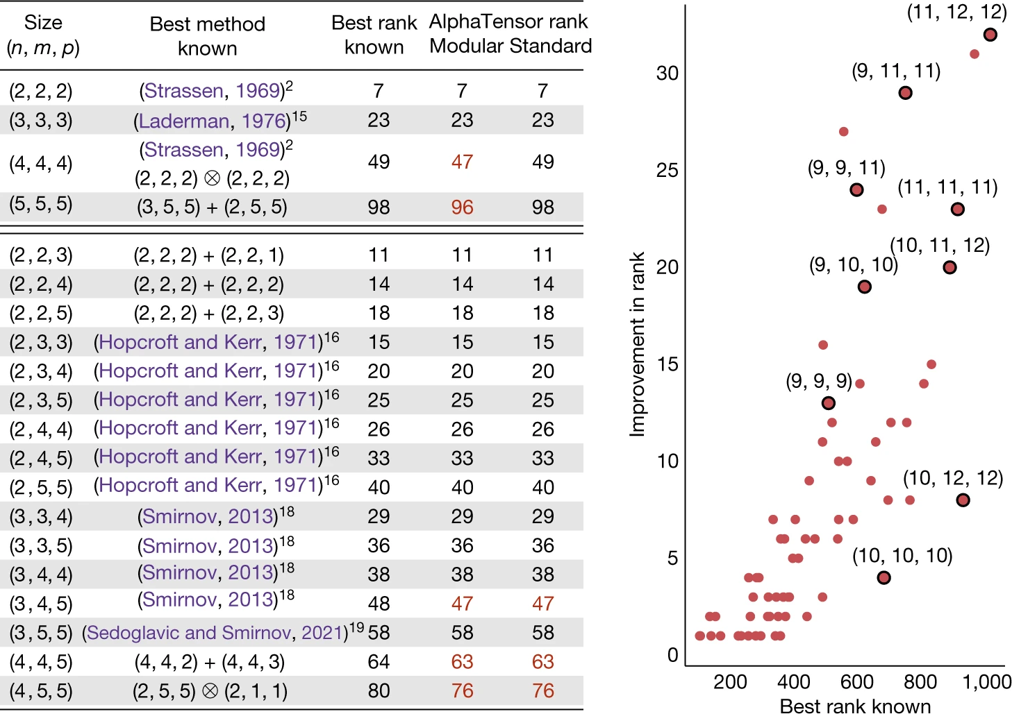
In all cases, AlphaTensor discovers algorithms that match or exceed existing State of the Art approaches.
Footnotes
Vassilevska Williams et al. "A Refined Laser Method and Faster Matrix Multiplication." October 13, 2020. CM-SIAM. ↩
Roth/Martin. "Computer Organization and Design: Integer Arithmetic." University of Pennsylvania ↩ ↩2
Coppersmith and Winograd. "Matrix multiplication via arithmetic progressions." January 1987. Association for Computing Machinery ↩
Alman, Josh. "Limits on the Universal Method for Matrix Multiplication." 2019. Theory of Computing, Vol. 17. ↩
Schönhage, Arnold; Strassen, Volker. "Schnelle Multiplikation großer Zahlen" [Fast multiplication of large numbers]. Computing. Vol. 7. ↩
Le Gall, François. "Powers of Tensors and Fast Matrix Multiplication." ISSAC 2014. https://arxiv.org/abs/1401.7714 ↩
Alhussein Fawzi et al. "Discovering faster matrix multiplication algorithms with reinforcement learning." October 5, 2022. Nature, vol. 610. ↩