Notes on Category Theory
- Published on
- ∘ 118 min read ∘ ––– views
Preface
This is a collection notes on Category Theory for personal reference.

Index
Glossary
Quick Definitions
Category Theory for Programmers
1 | Category: The Essence of Composition
2 | Types and Functions
3 | Categories, Great and Small
4 | Kleisli Categories
5 | Products and Coproducts
6 | Simple Algebraic Data Types
7 | Functors
8 | Functoriality
9| Function Types
10 | Natural Transformation
11 | Declarative Programming
12 | Limits and Colimits
Glossary
| Term | Definition |
|---|---|
| Monad | |
| Monoid | |
| Functor | |
| Endofunctor | |
| Category |
Quick Definitions
- A Category consists of
- A class called the class of object of
- A class is a collection of things which would yield a paradox if we called it a set
- For all , a class called the hom-set of morphisms (or maps, arrows) from to
- The homset is literally the collection of morphisms
- For all , a function , such that called composition
- For all , a morphism called the identity on
- Where composition is subject to the following conditions for all :
- For all morphisms , and , we have associativity:
- For all morphisms , we have
- A class called the class of object of
- A Functor between categories consists of where
- A function , such that
- For all , a function such that
- The function on morphisms is subject to the following conditions :
- If and , then . That is, preserves compositions
- Similarly, , so preserves identities as well
- Functors take objects to objects and morphisms to morphisms subject to sensible composition laws
- Forgetful functors take objects to a superclass of themselves by dropping some properties of the initial subclass
Classes of sameness
| class | |
|---|---|
| Equality | the same |
| Isomorphic | basically the same |
| Equivalence | basically basically the same |
| Naturally Isomorphic | Basically the same, but spicy |
| Adjunction | TODO |
Category Theory for Programmers
1 | Category: The Essence of Composition
- A category consists of objects and arrows that go between them
- The essence of a composition is a category, and vice versa (the essence of a category is composition)
TODO illustration
1.1 Arrows as Functions
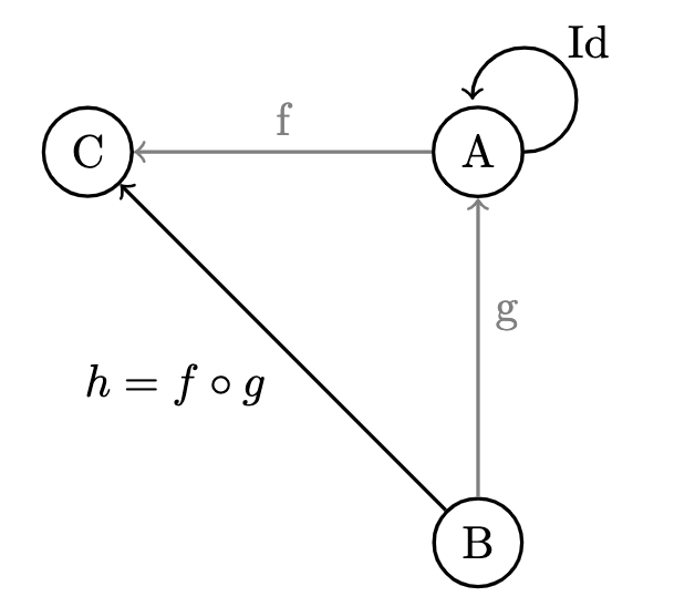
Arrows are morphisms, which, for the time being, can be thought of as functions (functions are a subset of morphisms).
If we have two functions and , then we can compose them to have a function given by where , unix pipe operator, and can be read as " of " or " after ."
1.2 Properties of Composition
- Composition is associative: it can be expressed without parentheses
- For every object , there exists and arrow which is a unit of composition. This arrow goes from the object back into itself. "Unit of composition" means that, when composed with any arrow that either starts or ends at , it will give back the same arrow. The unit for is the identity operation on given by , which is useful for higher order functions and establishing other properties of categories. Given a function ,
1.3 Composition is the Essence of Programming
- Programming naturally follows the technique of de-composing a large problem into smaller, digestible problems for efficient solutions.
2 | Types and Function
2.1 Who needs Types?
- Higher level languages' compilers protect from lexical and grammatical errors that might arise from arbitrary sequences of machine code
- Type checking is one mechanism to prevent non-sense programs
- Dynamically-typed languages resolve mismatches at runtime
- Statically-typed languages resolve mismatches at compile time
2.2 Types Are About Composability
- Category Theory is about composing arrows, but not just any combination of arrows, typically they have to compose between arrows of similar type
- Target object must be the same as the source of the next arrow
2.3 What are Types?
- Intuitively, we can think of types as sets of values e.g.,
- Types can be finite, like the set of allowable characters in a programming language:
- Types can be infinite:
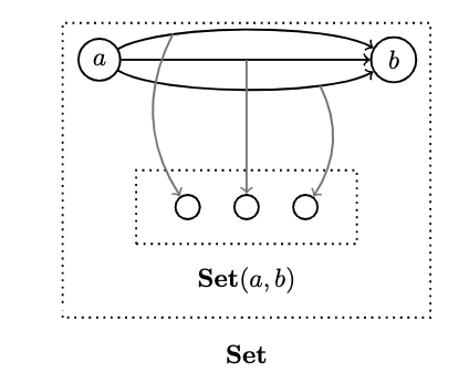
Set is itself a category where objects are sets, and morphisms or arrows are functions
A conflict which arises between the mathematical and programming understandings of the term "functions"
- A mathematical function is and answer
- A programming function is a sequence of executable steps to compute an answer. This is fine as long as there are finite steps, but recursive functions may never terminate
- Well-defined recursive definitions are fine, but determining whether a recursive functioning terminates is undecidable and has several neat implications.
Programming languages circumvent this by having all types extend a special value known as the bottom: which means non-terminating computation
For example, take the following Haskell function:
f :: Bool -> Bool
It might return True, False, or bottom. It's convenient to treat every runtime error as a bottom:
f x = undefined
which is acceptable to the type checker since undefined evaluates to bottom which is a member of any type including Bool.
- Functions that may return bottom are called partial, as opposed to total which returns valid values for all input arguments.
Because of this definition, the category of Haskell types and functions used above are called Hask, rather than Set. There's a theoretical distinction, but pragmatically speaking, they're equivalent
2.4 Why Do We Need a Mathematical Model?
It's hard to nail down precise semantic standards for programming languages
Operational Semantics represent a formal tool of describing behavior, but it's complex and academic
- Relies on / defines an idealized program interpreter
- It's rather difficult to prove program behavior this way since you have to run a program through your idealized interpreter to document a property which is only a minor improvement over how humans do it in our heads. And we all know how great we are at writing sound programs!
Semantics of industrial languages are usually described with informal operational reasoning in terms of an "abstract machine"
Denotational Semantics - a formalization under which every programming construct is given a mathematical interpretation. Languages which lend themselves to denotational semantics are "good" and those that don't are "bad" (I'm heavily paraphrasing here lol):
Consider the following programs
factorial n = product[1..n]
int factorial(int n) {
  int i;
  int res = 1;
  for (i = 2; i <= n; ++i)
    res *= i;
  return res;
}
This is something of a cheap shot since we could just as easily ask for a mathematical model of reading characters from stdin, or sending a packet across the wire, or any other program which doesn't intuitively lend itself to notation like that of computing the factorial of a number. GG Haskell.
The solution: Category Theory. Eugenio Moggi found that computational effect can be mapped to Monads which helps ?
2.5 Pure and Dirty Function
Recall that a mathematical function is just a mapping of values. Mathematical functions can easily be implemented as programming functions e.g. we can expect that a
squarefunction will produce the same output every time, regardless of outside factors- Squaring a number should not have the side effect of dispensing a dog treat, else it cannot be easily modeled as a mathematical function
A Pure Function always produces the same output when given the same input
- All functions in Haskell are pure, which contributes to why it's easier to describe the language's behavior with denotational semantics
A Dirty Function is one which produces side effects like dog treats by creating or relying upon external, (global) state
2.6 Examples of Types
2.6.1 Empty
- Is there a type that corresponds to the empty set?
- Not the C/C++
void, but yes the HaskellVoidsince it's a type that is not inhabited by any values, which nicely corresponds to the mathematical notion of . - Thus, you can define a function which accepts
Voidas an argument, but you can never invoke it since, by definition, no values satisfy the argument signature! - This function can happily return any type since it will never be called
absurd :: Void -> a
- Void represents falsity,
absurdcorresponds to the statement that from falsity follows anything
Ex falso sequitur quodlibet.
2.6.2 Singleton
- This is the C/C++
voidconstruct, holding only 1 possible value - A function from
voidcan always be called, and if it is pure, it will always return the same result
int f42() { return 42; }
The above example isn't quite taking "nothing" as the argument since "nothing" is Haskell's
Void, but since there's only one instance ofvoidin C/C++, it's implied in the function signatureHaskell's singleton is
()–the "unit"– which coincidentally results in a very similar signature:
f44 :: () -> Integer
f44 () = 44
- We can think of
f44is a substitute for the primitive Integer44which helps us express specific elements as functions or morphisms
2.6.3 void/Unit as a Return Type
- This is normally used for side-effecting functions, but these are not mathematical functions
- Formally, a function from set to Singleton set maps every element of to the single element of the Singleton. For all sets there exists one such function:
fInt :: Integer -> ()
fInt x = ()
fInt _ = ()
Note that it doesn't even depend on the type of argument
Functions that can be implemented with the same formula for any type like this are called parametrically polymorphic
unit :: a -> ()
unit _ = ()
2.6.4 Two-element Set
- In Haskell, the notion of
Boolis defined as
data Bool = True | False
- In libc it's a primitive (or if you're willing to suspend your pedantry, that is)
- Functions to the Boolean type are called predicates:
isEven,isNumeric,isTerminal, etc.
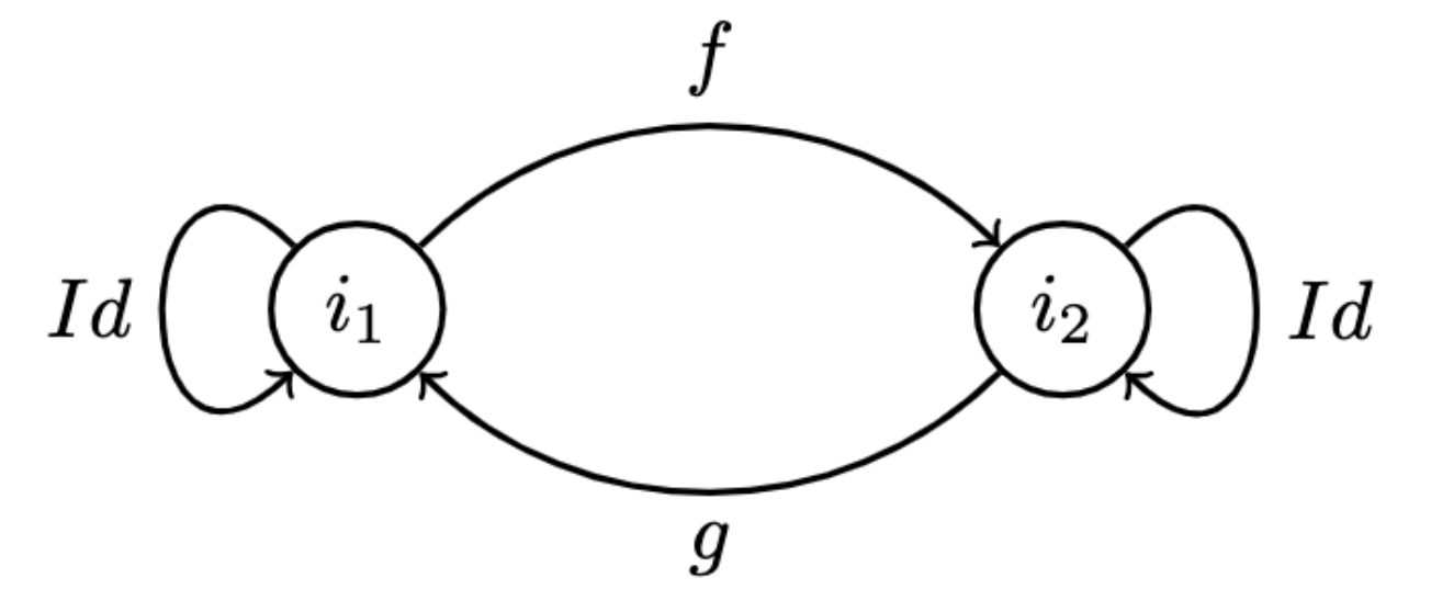
3 | Categories, Great and Small
3.1 - No Objects
- The category with zero objects consequently has zero morphisms
- It's important in the same way that the empty set, empty type, and the number 0 are important
3.2 - Simple Graphs
- Consider an arbitrary directed graph; we can make it into a category by adding a few more arrows:
- Ensure that each object has an arrow
- For any two arrows such that the end of one coincides with the beginning of another, add a new arrow to serve as their composition

- Here, we've created a category which has an object for all nodes in our graph, and all possible chains of composable graph edges as morphisms ( are special chains of length 0).
- This is an example of a free category generated by a graph and completed by extending it with the minimal number of items to satisfy its laws.
3.3 - Orders
- An Order is a category where a morphism is a comparative relation between objects
- We can verify that Orders are categories as follows:
- What's the identity in an Order? Every object is less than or equal to itself
- Can we compose objects in an Order? Yes, if and , then, transitively
- Is the composition associative? Also yes
- A set with this relation is called a Preorder which is a category
- A stronger conditional relation where
is known as a Partial Order
Lastly, imposing the condition that any two objects are in relation with each other yields a Linear Total Order
A Preorder is a category where there is at most one morphism from any object to object
- This is called a "thin" category
- A set of morphisms from objects to in a category is called a Hom-set and is denoted: or
- Every Hom-set in a preorder is either empty or a singleton
- This includes the Hom-set , the set of morphisms from to which must be the singleton containing only the identity
- There may be cycles in a preorder, but not a partial order
- Sorting algorithms like quicksort, mergesort, selection sort, etc. can only work on total orders
- Partial orders can be topologically sorted
3.4 - Monoid as Set
- A monoid is a set with an associative, binary operation and one special element that behaves like a unit with respect to this operation
- E.g., the natural numbers with zero form a monoid under addition. To verify:
- Associativity:
- neutral element: and
- The 2nd equation appears redundant because addition is commutative, but commutativity is not a requisite property of monoids, so it's included for thoroughness
- Another example, Strings form a monoid with the binary concatenation operation where the unit is the empty string which can be joined on either side of another string without modifying it
class Monoid m where
  mempty  :: m
  mappend :: m -> m -> m
First, what does the m -> m -> m argument list mean? It can be interpreted as:
- a function with multiple argument where the last, or rightmost, argument signifies the return type
- or as a function with one argument (leftmost) that returns a function. This can be hinted using parentheses e.g.
m -> (m -> m)but is redundant since arrows are right-associative
We can instantiate a string as an instance of Monoid and define its behavior:
instance Monoid String where
  mempty  = ""
  mappend = (++)
- Note that there are different paradigms for what equality means in programming languages:
- functional equality: what we have here,
mappend = (++), which is the equality of morphisms in the Hask category- Also known as point-free equality: equality without specifying arguments
- extensional equality:
mappend s1 s2 = (++) s1 s2, which is also known as point-wise equality, where the value of the functionmappendat point(s1, s2)is equivalent to(++) s1 s2
- functional equality: what we have here,
3.5 - Monoid as Category
Every monoid can be described as a single object with a set of morphisms that follow appropriate rules of composition
We can always extract a set from a single object category. This set is the set of morphisms. I.e., we have the Hom-set of the single object in the category
- We can easily define a binary operator in this set: the monoidal product of two set-elements. Given 2 elements of corresponding to and , their product will be equivalent to and this composition always exists because the source and target of the morphism are the same object .
- It's associative, and the identity morphism is the neutral element of the product, so we can always recover a set monoid from a category monoid, they're effectively equivalent.
Note that morphisms don't have to form a set; categories are broader than sets. In fact, a category in which a morphism between any two objects forms a set is called "locally small"
Elements of a Home-set can be seen as both
- morphisms which follow the rules of composition
- points in a set
Composition of morphisms in translates into a monoidal product in the set .
4 | Kleisli Categories
- How can we model non-pure functions or side effects in Category Theory?
- Imperatively, this is achieved by modifying global state
string logger;
bool negate(bool b) {
  logger += "Not so!";
  return !b;
}
- This function is not pure since its memoized version fails to produce a log. A more modern approach might resemble the following:
Pair<bool, string> negate(bool b, string logger) {
  return make_pair(!b, logger + "Not so!");
}
- This still sucks from a design perspective. It would be better to aggregate the log message externally between function calls:
Pair<bool, string> negate(bool b) {
  return make_pair(!b, "Not so!");
}

res = negate(true);
negated = res.first;
logger += res.second;
- But, externally aggregating all logs is gross, and we can abstract this repetition further, but then we'd be abstracting the composition of functions 👻
4.1 - Writer Category
- Embellishing return types of functions is very useful. We start with a regular category of types and functions. We leave types as our objects, but we redefine our morphisms to be the embellished functions
- E.g., We want to embellish
isEvenwhich goes frominttobooland turn it into a morphism that is represented by an embellished function- This morphism would still need to be considered an arrow between objects
int,bool, even though the embellished function returnsPair
- This morphism would still need to be considered an arrow between objects
Pair<bool, string> isEven(int n) { return make_pair(n % 2 ==0, "isEven"); }
- By laws of categories, wee should be able to compose this with another morphism that goes from object
boolto whatever:
Pair<bool, string> negate(bool b) { return make_pair(!b, "Not so!"); }
The literal composition would look like:
Pair<bool, string> isOdd(int n) {
  Pair<bool, str> p1 = isEven(n);
  Pair<bool, str> p2 = negate(p1.first);
  return make_pair(p2.first, p1.second + p2.second);
}
The formula for composition, then, is:
- Execute the embellished function corresponding to the first morphism
- Extract the first component of the result and pass it to the second morphism
- Concatenate the second component of the first result with the second component of the second result.
- Return the new pair combining the first component of the final result with the concatenated result from (3)
- If we want to abstract this composition, we just need to parameterize the three object involved in our category: two embellished functions that are composable according to our rules, and return the third embellished function.
template<class A, class B, class C>
function<Writer<C>(A)> compose(function<Writer<B>(A)> m1,
                               function<Writer<C>(B)> m2) {
  return [m1, m2](A x) {
    auto p1 = m1(x);
    auto p2 = m2(p1.first);
    return make_pair(p2.first, p1.second + p2.second);
  }
}
4.2 - Writer in Haskell
type Writer a = (a, String) -- alias/typedef, parameterized by a
a -> Writer b -- morphisms
We declare the composition of Writers using Haskell's "fish" operator which is a function of two arguments which are other functions and returns a function
(>=>) :: (a -> Writer b) -> (b -> Writer c) -> (a Writer c)

m1 >=> m2 = \x ->
  let (y, s1) = m1 x
      (z, s2) = m2 y
  in (z, s1 ++ s2)
with the identity:
return :: a -> Writer a
return x = (x, "")
Then, we can compose them:
upCase :: String -> Writer String
upCase s = (map toUpper s, "upCase")

toWords :: String -> Writer [String]
toWords s = (words s, "toWords")

process :: String -> Writer [String]
process = upCase >=> toWords
4.3 - Kleisli Categories
Based on Monad, where:
- Objects are the types of the underlying programming language
- Morphisms from types to are functions that go from to a type derived from using the particular embellishment
- Later, we'll see that "embellishment" is an imprecise description of the notion of an endofunctor is a category
The last degree of freedom is composition itself which is precisely what makes it possible to give denotational semantics to programs that, in imperative languages, are traditionally implemented with side effects.
5 | Products and Coproducts
- In Category Theory, there exists a common construction called the "Universal construction" for defining object in terms of their relationships (morphisms)
- Pick a pattern or shape constructed from objects and arrows and look for all its occurrences in the category
- For large enough categories and common enough shapes/patterns, we can find many instances. We can establish a ranking over them and pick what is considered to be the best fit, like a search engine. The line to toe is
- generality: large recall
- specifcity: precision
5.1 - Initial Object
- This is the simplest shape. There are as many instance of this shape as there are objects in a given category
- We need to rank them, and all we have are morphisms
- It is possible that there is an "overall net flow" of arrows from one end of the category to the other, especially in (partially) ordered categories
- We can generalize the notion of object precedence by saying that " is more initial than " if there is an arrow from to :
- "The" initial object is one that has arrows going to all other objects
- There is no guarantee that such an object exists in an arbitrary category, but that's okay.
- The bigger problem is that there might be too many objects matching this description (good recall, low precision)
- Leveraging ordered categories which have implicit restrictions on morphisms between objects: there can be at most one arrow between objects since there is only one way of being less than or equal to another object, we get a definition of the initial object: The object that has one and only one morphism going to any object in the category
- Even this doesn't guarantee uniqueness of the initial object though (if it exists), but it does guarantee uniqueness up to isomorphism.
- There is no guarantee that such an object exists in an arbitrary category, but that's okay.
Examples:
- Within a partially ordered set (poset): initial object is the the least object
- Category of sets and function: empty set (Haskell's
Void) and the unique polymorphic function:
absurd :: Void -> a
5.2 - Terminal Object
Similarly, we can identify an object which is "more terminal" than
The Terminal Object is the object with exactly one incoming morphism from any other object in the category
- The terminal object is also unique up to the point of isomorphism
- In a poset, the terminal object is the "biggest" object
- In the category of sets and functions, it's a singleton
- In Haskell, it's the unit
(), and in C/C++ it'svoid
Earlier, we established that there is only one pure function from any type to the unit type:
unit :: a -> ()
unit _ = ()
Here, uniqueness is critical, because there are other sets (all of them, actually, except for the Empty category) that have incoming morphisms from every set.
- There exists a boolean function (predicate) defined for every type:
yes :: a -> bool
yes _ = True
But this isn't the/a terminal object, because there's at least one more:
no :: a -> bool
no _ = False
- Insisting on uniqueness gives us just the right amount of precision to narrow down the definition of the terminal object to just one type
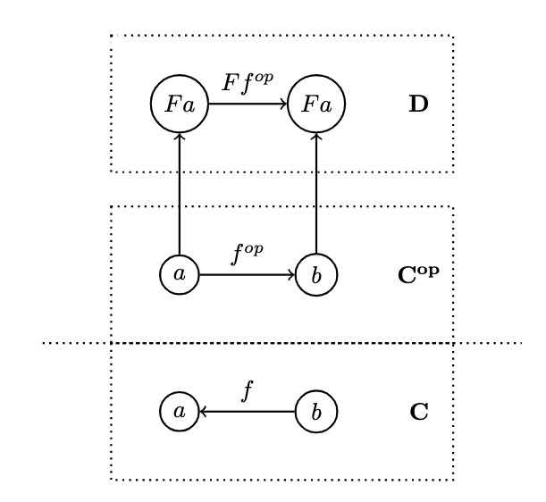
5.3 - Duality
- Observing the symmetry between definitions of initial and terminal objects, we can reason that: for any category, we can define the opposite category: , just by reversing all the arrows
- This automatically satisfies all the requirements of a category as long as we simultaneously redefine composition. If the original morphisms
f :: a -> b
g :: b ->
-- composed to
h :: a -> c
with , then the reversed morphisms must be and and will compose to , .
Reversing the identity morphisms is a no op:
- Duality doubles the "productivity" as, for all categories once concocts, there exists the dual category you get for free!
5.4 - Isomorphisms
Intuitively it means, "they look the same." That is, every part of corresponds to
Formally, it means that there exists a mapping from and back, , and they (the mappings) are the inverse of one another
Inverse here is defined in terms of composability and identity:
- a morphism is the inverse of if their composition is the identity: and
Recall that the initial and terminal objects are unique up to isomorphism. This is because any two initial or terminal objects are isomorphic.
For example, take two initial object . Since is initial, there exists a unique morphism from . By the same reasoning, we have .

- Note that all morphisms here are unique.
- The composition of must be a morphism from , but is initial, so there can only be one morphism from .
- Since we are in a category, we know there is an identity morphism from , and since there can only be one, that must be it (the identity).
- Therefore, , similarly since there exists only one morphism from .
- Therefore and must be inverses of one another, so two initial objects are isomorphic
- Not that and must be unique in this proof because not only is the initial object unique up to isomorphism, but it is unique up to unique isomorphism.
- There could be multiple isomorphisms between two objects
5.5 - Products
- Recall that the Cartesian product of two sets is the set of all pairwise combinations therein:
- How can we generalize this pattern that connects the product set with its constituent sets?
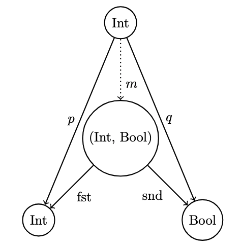
- In Haskell, we have two functions, the projections, from the product to each constituent:
fst :: (a, b) -> a
fst (x, _) = x

snd :: (a, b) -> b
snd (_, y) = y
- With even this limited vocabulary, we can construct the product of two sets which consists of an object and two morphisms connecting it to and respectively:
p :: c -> a
q :: c -> b

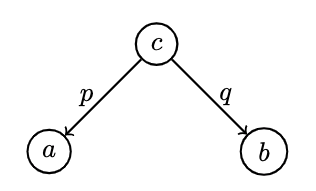
- All 's which fit the pattern can be considered candidates for the product, there might be multiple:

For example, we can define two Haskell types as our constituents, Int, Bool:
p :: Int -> Int
p x = x

q :: Int -> Bool
q _ = True
Which, as it stands, is pretty lam, but matches our criteria. Consider a denser, but also satisfactory pair of constituent types:
p :: (Int, Int, Bool) -> Int
p (x, _, _) = x

q :: (Int, Int, Bool) -> Bool
q p (_, _, b) = b
Whereas the first set of projections was too small, only covering the Int dimension of the product, these candidates are too broad, with the unnecessary duplicate Int dimension.
Returning to the universal ranking, how do we compare two instances of our pattern? That is, how do we evaluate
- We would like to say that is "better" than if there is a morphism from , but that constraint alone is insufficient. We also want its projections to be "better" or "more universal" than those of .
- We want to be able to reconstruct from and 's projections:

- This can be interpreted as " factorizes and ."
- Using the pair
(Int, Bool), with the two canonical projections / "vocabulary" introduced earlier:fst, sndare "better" than the other two candidates:

-- mapping for first, simple candidate
m :: Int -> (Int, Bool)
m x = (x, True)

-- reconstructions of projections
p x = fst (m x) = x
q x = snd (m x) = True
And in our second, more complex example, has a similar uniquely determined :
m (x, _, b) = (x,b)
Therefore, (Int, Bool) is better than either of the other two candidates. Why isn't the opposite true? That is, can we find some that would help reconstruct fst, snd from ?
fst = p . m'
snd = q . m'
In our first example, always returns
True, and we know that there exist pairs with second components that areFalse, which we can't reconstruct from as defined.In the second example, we return enough information after or , but there's multiple factorization of
fstandsndsince both and ignore the second component of the triple. Ourm'can put anything there:
m' (x, b) = (x, x, b)

-- or

m' (x, b) = (x, 42, b)
Thus, given any type with two projections , there is a unique from to the Cartesian product that factorizes them:
m :: c -> (a, b)
m x = (p x, q x)
which makes the Cartesian product our best match, which implies that this universal construction works in the category of Sets.
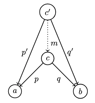
Now, let's generalize that same universal construction to define the product of two objects in any category.
Note that the product doesn't necessarily always exist, but when it does, it is unique up to unique isomorphism
A product of two objects and is the unique object equipped with two projections such that, for any other object equipped with two projects, there is a unique morphism from to that factorizes those projections
A higher order function which produces that factorizing function from two candidates is sometimes called the factorizer:
factorizer :: (c -> a) -> (c -> b) -> (c -> (a, b))
factorizer p q = \x -> (p x, q x)
-- \x is a lambda expression or anonymous function
- to summarize, products are ranked according to their ability to factorize the morphism of their competing product-candidate's projections
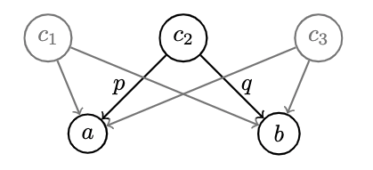
5.6 - Coproducts
- Like every construction in Category Theory, the product has a dual: the coproduct
- Reversing the arrows in the product pattern yields an object with two injections which are morphisms from respectively:

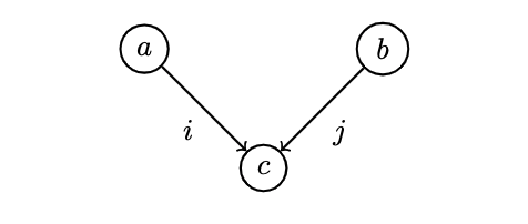
- The ranking of possible coproducts is also inverted such that is "better than" (also equipped with two injections ) if there is a morphisms from to which factorizes the injections:

- A coproduct of two objects is the object equipped with two injections such that for any other object equipped with two injections, there is a unique morphism from to that factorizes those injections.
- In the category of Sets, it is the disjoint union of two sets: an element of the disjoint union of is either an element of or an element of . If and overlap, then the disjoint union contains two copies of the common part (somehow skirting the definition of a set??)
- The skirting part happens by "tagging" the elements with an identifier that specifies the origin
- In the category of Sets, it is the disjoint union of two sets: an element of the disjoint union of is either an element of or an element of . If and overlap, then the disjoint union contains two copies of the common part (somehow skirting the definition of a set??)
In programming terms, it's represented as a union with the added field of a tag enum:
struct Contact {
  enum { isPhone, isEmail} tag;
  union {int phoneNum; char const* emailAddr; };
}
// with injections as "constructors" or functions:

Contact PhoneNum(int n) {
  /** this example is straight from the book,
      but this should be dynamically allocated 💅 **/
  Contact c;
  c.tag = isPhone;
  c.phoneNum = n;
  return c;
}
- Tagger unions are sometimes called variants
In Haskell:
data Contact = PhoneNum Int | EmailAddr String
helpdesk :: Contact
helpdesk = PhoneNum 9118675309
- Unlike the canonical implementation of product which is the primitive
Pair, Haskell's coproduct is a data typeEither:
data Either a b = Left a | Right b
- Just as we defined a factorizer for a product, we can define one for coproduct. Given a candidate type and two candidate injections , the factorizer for
Eitherproduces the factorizing function:
factorizer :: (a -> c) -> (b -> c) -> Either a b -> c
factorizer i j (Left a) = i a
factorizer i j (Right b) = j b
5.7 - Asymmetry
Despite the similarities between categories and their duals obtained by reversing morphisms, and similarity with initial / terminal objects in the category of sets, there are important qualities of these elements which are not symmetric:
- Product behaves like multiplication, with the terminal object playing the role of the multiplicative identity of one
- Coproduct behaves more like a sum, with the initial object playing the role of zero.
For finite sets:
- The size of the product is the product of the sizes of individual sets
- The size of the coproduct is the sum of the sizes
Therefore, the category of sets is not symmetric with respect to just inversion of arrows.
Other asymmetries include:
- Empty set: has a unique morphism to any set (the absurd function), but has no incoming morphisms
- Singleton set: has a unique morphism to it from every set, but it also has outgoing morphisms to every set (excluding the empty set)
- It is inherently tied to the product which is what sets it apart from the coproduct
Consider using this set, represented by the unit (), as yet another, vastly inferior candidate for the product pattern, equipped with two projections from the singleton to each constituent set. Because the product is universal, there is also a unique morphism from our unit candidate to the product.
Recall that select an element from the product set and factorizes the two projections:
p = fst . m
q = snd . m
When acting on the singleton value, the only element is (), so these become:
p () = fst (m ())
q () = snd (m ())
Conversely, there is not an intuitive interpretation of how this behaves for the coproduct, since the unit () tells us nothing about the source of the injections.
This is a property of functions, not sets. Functions in general aree asymmetric.
- A function must be defined for every element in its domain.
- In programming language, it's a total function.
- But, it doesn't have to cover the whole codomain or range
- When the size of the domain is substantially less than that of the codomain, we think of such functions as embedding the domain in the codomain.
- I.e. from a singleton is embedded in the codomain
- Formally, these are referred to as surjective/onto: functions that tightly fill their codomains
- A function that maps an element to every element that is, for every , there is an such that
- Another source of asymmetry is that functions are allowed to map many elements of the domain set into one element of the codomain
- I.e. the unit collapses a whole set into a singleton. Collapsing in this way is composable, and the results of composing collapsing operations are compounded
- These functions are called injective or one-to-one
- Bijections are the middle child of classes of functions in that they are symmetric because they are invertible. Isomorphisms in category theory are equivalent to bijections
6 | Simple Algebraic Data Types
- Many common data structures can be built using the two Algebraic Data Types covered so far: product, coproduct
- For composite types (types construct from primitives), equality, comparison, conversion, and more can be derived from the properties of products and coproducts
6.1 - Product Types in Programming
- Canonically a a product in Haskell is a primitive
Pair, in C++, it's a template from the stdlib- Pair's aren't strictly commutative, meaning that
(Int, Bool)is not necessarily equivalent to(Bool, Int), but they are commutative up to the isomorphism given by aswapfunction:
- Pair's aren't strictly commutative, meaning that
swap :: (a, b) -> (b, a)
swap (x, y) = (y, x)
- We can generalize the swap function for nested types since the different ways of nesting
Pairs are isomorphic to one another. E.g., nesting a product triple ofa, b, ccan be achieved two ways:(a, (b, c))and((a, b), c)- These are different types, but their elements are in 1:1 correspondence and we can map between them:
alpha :: ((a, b), c) -> (a, (b, c))
alpha ((x, y), z) = (x, (y, z))
which, like swap, is also trivially invertible
The creation of a product type can be interpreted as a binary operation on types. Thus, the alpha isomorphism looks very similar to the associativity law for monoids:
Except that in the monoid case, these two compositions were equal, whereas here they're only equal up to isomorphism
- If we're content with equality up to isomorphism (which we are), and don't need strict equality (which we don't), we can go even further and show that the unit type
()is the unit of the product in the same way that is the unit of multiplication.- Pairing a value type with a unit doesn't add any information, e.g.,
(a, ())is isomorphic toavia:
- Pairing a value type with a unit doesn't add any information, e.g.,
rho :: (a, ()) -> a
rho (x, ()) = x

-- inverted by

rho :: a -> (a, ())
rho x = (x, ())
- Formally, the category of sets is a monoidal category because we can multiply objects by taking their Cartesian product
6.2 - Record
Example: We want to design a representation for a chemical element, and be able to verify that a chemical's symbol corresponds to the prefix of its name:
startwithsymbol :: (String, String, Int) -> Bool
startwithsymbol (name, symbol, _) = isPrefixOf symbol name
But this is bad, error prone, and reliant on contextual clues. A better model might resemble:
data Element = Element {
                         name :: String,
                         symbol :: String,
                         atomicNo :: Int
                        }
These two representations are isomorphic as evidenced by some conversion functions:
tupleToElem :: (String, String, Int) - Element
tupleToElem (n, s, a) = Element { name = n, symbol = s, atomicNo = a }

elemToTuple :: Element -> (String, String, Int)
elemToTuple e = (name e, symbol e, atomicNo e)
-- names of data fields serve as getters to access those fields
We can clean up our initial attempt at modeling a chemical as follows
startwithsymbol :: Element -> Bool
startwithsymbol e = isPrefixOf (symbol e) (name e)
6.3 - Sum Types
- Just as the product in the category of sets gives way to product types, coproducts correspond to sum types, canonically expressed as
Eithertypes- They are also commutative up to the point of isomorphism and
- nestable up to the point of isomorphism (e.g., we can have a triple as a sum)
data oneOfThree a b c = Sinistral a | Medial b | Dextral`
Set is also a symmetric monoidal category with respect to coproduct where
- the binary operation is disjoint sum:
Either - the unit element is the initial object:
Void - Accordingly,
Either a Voidis equivalent toasince it's not possible to construct a value of typeVoid: - Sums are common in Haskell / FP
- Less so in imperative languages, though they can be represented as variant unions (tagged unions)
- Enums usually suffice, or primitives like
stdbool.h
- the binary operation is disjoint sum:
Sum types which communicate the presence or absence of value or represented in Haskell as
data Maybe a = Nothing | Just a
--             ()        encapsulates a
- Immutability in FP allows repeated use of constructors for pattern matching in the reverse language
6.4 - Algebra of Types
- While powerful alone, combining the product and sum types via composition yields even richer types
- We have two commutative monoidal structures underlying our small type system so far:
- Sum with
Voidas the neutral element representing - Product with
()as the neutral element representing
- Sum with
- Do these follow the expected rules of arithmetic like ?
- Is a product with one component being
Voidisomorphic toVoid? Can we create a Pair of(Int, Void)? - We need two values; we can take any
Intfor the first component of the Pair, but there are no values of typeVoid, so the type(Int, Void)is also uninhabited, which is equivalent toVoid - ✅
- Furthermore, the distributive property also follows from this:
- Is a product with one component being
    a * (b + c) = a * b + a * c
(a, Either b c) = Either (a ,b) (a, c)
given by
prodToSum :: (a Either b c) -> Either (a, b) (a, c)
prodToSum = (x, e) = case e of
                      Left y  -> Left (x, y)
                      Right z -> Right (x, z)

sumToProd :: Either (a, b) (a, c) -> (a, Either b c)
sumToProd e = case e of
                Left (x, y)  -> (x, Left y)
                Right (x, z) -> (x, Right z)
- Two such intertwined monoids are called semi-rings (semi because we can't/haven't defined subtraction or division on types)
- Interpreting semi-ring types as natural numbers yields the following correspondences
| Expression | Type | | ------------ | --------------------------------- | -------- | | | Void | | | () | | | Either a b = Left a | Right b | | | (a, b) or Pair a b = Pair a b | | | data Bool = True | False | | | data Maybe = Nothing | Just a |
Listis defined as a recursive solution to an equation:
data List a = Nil | Cons a (List a)
-- `Cons` is a historical holdover name from Lisp for Constructor
If we do some algebraic substitutions using the table above and replace List a with , and we get:
But, because we're working with a semiring, we can't solve this equation with division or subtraction. Instead, we'll keep replacing with :
An infinite sum of product tuples which can be:
an empty list,
a singleton
a pair of
a triple of (a _ a _ a), etc.
The product of two types must contain both a value of type and a value of type ; they both must be inhabited
Sums can contain either a value for type or type , but both are not required
Logical and and or also form a semiring and can be mapped to Type Theory:
| Expression | Type | | ---------- | -------------------- | -------- | | | Void | | | () | | | Either a b = Left a | Right b | | | (a, b) |
- Logical types and natural numbers are isomorphic via types
7 | Functors
- A Functor is a mapping between categories
- Given two categories , a functor maps objects in to objects in
- If is an object in , we write its image in as
- A functor also maps morphisms –it's function on morphisms, but it doesn't just map morphisms willy nilly– it preserves connections
- If A morphism in connects , () then the image of in will connect the image of to the image of :

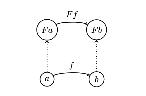
- Functors preserve the structure of a category: what's connected in one category is connected in another
- We also need to preserve the composition of these morphisms. E.g., if we have , we want its image under to be a composition of the images of

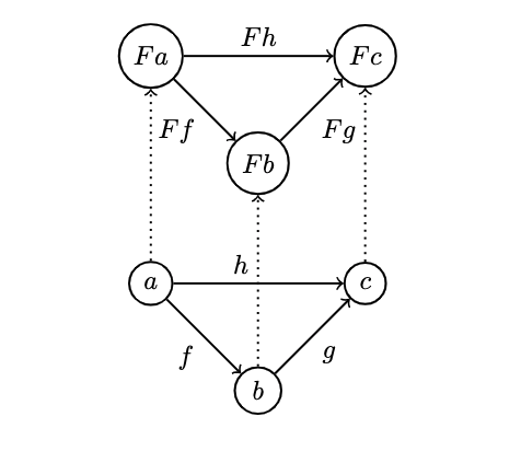
- Finally, we want all identity morphisms in to be mapped to the identity morphisms in :
where is the identity at object and is the identity at .
- Not that functors are more restrictive than regular functions in that they must preserve the structure of the program. They can't introduce and "tears," but they can "combine" morphisms.
- This restriction is roughly analogous to the occasional requirement of continuity of functions in calculus
- Functors can also collapse and embed, just like functions as described earlier, where embedding is more prominent when the source category is smaller than the target category; I.e., the source being the Singleton, and the target is any other arbitrary Category (excluding the empty category, of course)
- A functor from a singleton to any other category will just select an object from the target, just like a morphisms from a singleton set
- The maximally collapsing functor is called the constant , which maps every object in the source category to one object in , the target, and also maps every morphism in the source to the identity
- It's like a black hole
7.1 - Functors in Programming
- We have the category of types and functions
- An endofunctor of this category maps to the category itself
7.1.1 - The Maybe Functor
Recall the Maybe doohicky:
data Maybe a = Nothing | Just a
Here, Maybe is not a type, but a type constructor. It needs a type argument to be a type, otherwise it's just a function on types
For example, for any function from a to b:
f :: a -> b
we want to produce a function
Maybe a -> Maybe b
- In the case of having
Nothingin theMaybe, we just returnNothing - In the case of
Just, we applyfto its contents such that the image offunderMaybeis
f' :: Maybe a -> Maybe b
f' Nothing = Nothing
f' (Just x) = Just (f x)
- In Haskell, we can implement the morphism-mapping part of a functor as a higher order function call
fmap, which would resemble the previous case:
fmap :: (a -> b) -> (Maybe a -> Maybe b)

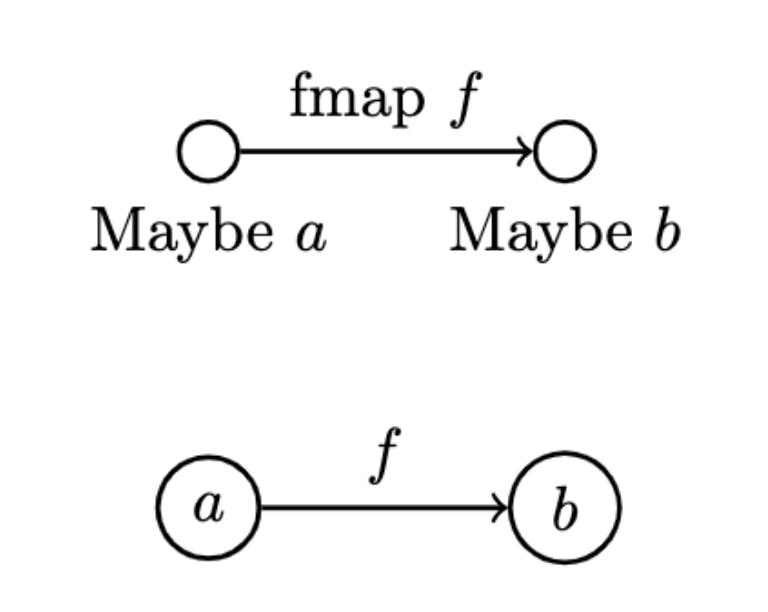
- We say that a
fmaplifts a function - To show that the type constructor
Maybealong with thefmapfunction forms a functor, we have to show thatfmappreserves both identity and composition: the Functor Laws
7.1.2 - Equational Reasoning
- Equational reasoning is a means of proof which relies on substitution. I.e., base on the definition of
fmapgiven above, if we saw an expression likefmap f Nothing, we could replace it with justNothing - Using this to show that
fmappreserves identity we get:
fmap id = id -- which has two cases

-- case Nothing
fmap id Nothing = Nothing      -- the definition of fmap
                = id Nothing   -- definition of id

-- case Something
fmap id (Just x) = Just (id x) -- definition of fmap
                 = Just x      -- definition of id
                 = id (Just x) -- definition of id
- Then, to show preservation of composition:
fmap (g . f) = fmap g . fmap f

-- case Nothing
fmap (g .f) Nothing = Nothing        -- definition of fmap
                    = fmap g Nothing -- definition of fmap
                    = fmap g (fmap f Nothing)
                                     -- definition of fmap

-- case Something
fmap (g .f) (Just x) = Just ((g . f) x)    -- definition of fmap
                     = Just (g (f x))      -- definition of composition
                     = fmap g (Just (f x)) -- definition of fmap
                     = fmap g (fmap f (Just x))
                                           -- definition of fmap
                     = (fmap g . fmap f) (Just x)
                                           -- definition of composition
7.1.3 - Optional
- Ugly sketch of an implementation in c++
7.1.4 - Typeclasses
- How do we abstract the functor
- This is an utterly psycho question. Where do you draw the line bruh
- Typeclasses define a family of types that support a common interface
For example, the class of objects which support equality:
class Eq a where
  (==) :: a -> a -> bool

data Point = Pt Float Float
instance Eq Point where
  (Pt x y) == (Pt x' y') = x == x' && y == y'
- Problem: a functor is not defined as a type, but as a mapping of types... But Haskell typeclasses work with type constructors as well as types:
class Functor f where
  fmap :: (a -> b) -> fa -> fb
Here, f is a functor, and if there exists an fmap w that type signature, then the Haskell compiled can deduce that f is a type constructor, not a type
instance Functor Maybe where
  fmap _ Nothing = Nothing
  fmap f (Just x) = Just (f x)
7.1.5 - Functor in c++
- I sleep
7.1.6 - The List Functor
- Any type that is parameterized by another type is a good candidate for to be a functor, I.e., most generic collections
data List a = Nil | Cons a (List a)
- To show that
Listis a functor, we have to define the lifting functions: given a functiona -> b, define a functionList a -> List b
fmap :: (a -> b) -> (List a -> List b)
which also has two cases:
Nil: easy, since there's not much to do with an empty listCons List a: a bit tricky with recursion:- We have a list of
a, a functionfthat turnsa -> b, and we want a list ofb - The constructor
Consjoins the head of a list with the tail - We apply
fto the head and apply the liftedfto the tail
- We have a list of
fmap f (Cons x t) = Cons (f x) (fmap f t)
-- this is recursively bound by the necessarily shrinking
-- portion of the list until we reach Nil and we have
-- previously defined: fmap f Nil = Nil, which will terminate
All together then:
instance Functor List where
  fmap _ Nil = Nil
  fmap f (Cons x t) = Cons (f x) (fmap f t)
7.1.7 - Reader Functor
Consider a mapping of type
ato the type of a function returninga- Mappings of function types are coming down the road, but we have some programming intuition about function types
(a ->b)takesaand returnsband is equivalent to(->) a bJust like with regular functions, type functions of more than one argument can be partially applied such that when we provide just one type argument, it still expects another on, meaning that
(->) ais a type constructor, awaiting a typebto produce a complete type signatureThis defines a whole family of type constructors parameterized by
a.- Are they functors, though? Lets rename the argument type to be
rand the result type to beaso the typeConstakes any typeaand maps it to typer -> a. - To show that it's a functor, we need to lift a function
a -> bto a function(->) awhich returns(r -> b)(the types formed using the type constructor(-> r)acting ona, brespectively)
- Are they functors, though? Lets rename the argument type to be
fmap :: (a -> b) -> (r -> a) -> (r -> b)
Given a function
f :: a -> b
and
g :: r -> a
we want to create r -> b, and there is only one way to compose f, g and the result is r -> b
instance Functor ((->) r) where
  fmap f g = f . g -- equiv. to just fmap = (.)
7.2 - Functors as Containers
- The reader functor treats functions as data which should feel a bit abnormal, but recall that functions can be memoized and execution can be tabularizeed
- In may functional programming languages, traditional collections may be implemented as functions
naturals :: [Integer] -- built in type constructor
naturals :: [1..]     -- list literal, can't be stored in memory
                      -- but the compiler implements as a function that
                      -- generates ints on demand
Thus, we can blur the lines and move freely between code <--> data
- Think of the functor object (generated by an endofunctor) as containing a value or values of the type over which it is parameterized, even if those values are not physically present
- It may contain the value, or the recipe for generating those values
Futuremay have the value, maybe not- From a functor level, we don't care if we can access the values at any given time, just that they can be manipulated and composed properly
To illustrate that, let's define a type which completely ignores its argument
Data Const c a = Const c
fmap :: (a -> b) -> Const c -- I don't care, I don't
-- because functor ignores the argument,
-- the impl of fmap is free to ignore its function args

instance Functor (Const c) where
  fmap _ (Const v) = Cons v
Observe that the Constant functor is a special case of : the endofunctor case of the black hole
7.3 - Functor Composition
- Jsut as functions compose between sets, functors compose between categories
- Recall the
maybeTailexample:
maybeTail :: [a] -> Maybe [a]
maybeTail [] = Nothing
maybeTail (x:xs) = Just xs
- What if we want to apply some
fto the contents of the compositeMaybe List?- We have to break through two layers of functors.
fmapbreaks through the outer,Maybelater, but we can't just sendfinsideMaybebecause it doesn't work on Lists. We have to send(fmap f)to operate on the inner list:
- We have to break through two layers of functors.
For example, if we want to swuare the elements of a Maybe List:
square x = x * x

ms :: Maybe [Int]
ms = Just [1, 2, 3]

ms2 = fmap (fmap square) ms
The compiler will recognize that he first, outer fmap pertains to the Maybe component, and the inner fmap to the List, which is also equivalent to
ms2 = (fmap . fmap) square ms
-- since a functor can be considered a function with one arg:
fmap :: (a -> b) -> (f a -> f b)
-- and in our case, the 2nd fmap in (fmap . fmap) takes as its argument
square :: Int -> Int
-- and returns
[Int -> Int]
-- first fmap then takes that function and returns a function
Maybe [Int] -> Maybe [Int]
-- finally, that function is applied to ms
- It's obvious that functor composition is associative and that there exists a trivial identity functor in every category which maps every object to itself, and every morphism to itself
- So, functors have all the same properties as morphisms in some category
- But what category? It would have to be a category in which objects themselves are categories, and morphisms are functors; a category of categories!
- But, a category of all categories would have to include itself, and we get into the same kind of Set Theoretical paradoxes that make the Set of all Sets impossible
- There exists a category which contains all Small Categories called Cat (which itself is Big, so it can contain itself)
- All objects in a small category form a set, as opposed to something larger than a set
8 | Functoriality
- Building larger funcors from smaller functors (which correspond to mappings between objects in a category) can be extended to functors (which include mappings between morphisms)
8.1 - Bifunctor
- Since functors are morphisms in Cat, a lot of intuititons about morphisms can apply to functors as well
- A Bifunctor is a functor of two arguments on objects. It maps every pair of objects to an object in .
- In other words, it's a mapping from a Cartesian product of categories. This alone is straightforward, but functoriality means that a bifunctor also has to map morphisms

- A pair of morphisms is just a single morphism in the product category of , and these can be interpreted in the obvious way:
which is associative, has an identity and thus is a category
We could consider a bifunctor as two separate functors, checking each constituent argument. However, general, separate functoriality does not prove joint functoriality
- Categories in which joint functoriality fails are called pre-monoidal
In Haskell, we can define a bifunctor between three identical categories: namely, the category of Haskell types
class Bifunctor f where
  bimap :: (a -> c) -> (b -> d) -> f a b -> f c d
  bimap g h = first g . second h
  first :: (a -> c) -> f a b -> f c b
  first g = bimap g id
  second :: (b -> d) -> f a b -> f a d
  second = bimap id

- The type variable
frepresents the bifunctor. It's evident from all the type signature, it's always applied to two type arguments, and the result is a lifted function(f a b -> f c d), operating on types generated by the bifunctor's type constructor - There's a default implementation of
bimapin terms offirstandsecond, but this might not always be an available pattern because two maps may not commute (more on what the hell this means later, but for the time being):
The two other signatures of first and second are the two fmaps witnessing the functoriality of f in the first and second arguments of the bifunctor
First

Second

- When declaring an instance of bifunctor, you either have to define
bimapand accept the defaults forfirst, secondor implementfirst, secondyourself and accept the defaults forbimap
8.2 - Product and Coproduct Bifunctors
- A categorical product is a bifunctor. The simplest example is the bifunctor instance for a
Pairconstructor:
instance Bifunctor (,) where
  bimap f g (x ,y ) = (f x, g y)
which is preetty straightforward, bimap applies first to x and second to y
bimap :: (a -> c) -> (b -> d) -> (a, b) -> (c, d)
and the action of the bifunctor here is to make pairs of types:
(,) a b = (a, b)
and, by duality, a coproduct if its defined for every pair in the category, is also a bifunctor.
- We can now add to our definition of a Monoidal Category that the binary operator must be a bifunctor
8.3 - Functorial Algebraic Data Types
We can specify the construction of complex types from simpler types relying on the sum and product types (which we've just shown are functorial) as ADTs
What are the building blocks of parameterized ADTs?
- First, there are items with no dependency on the type parameter(s) of the function. For example, , , or any other form of our
Constfunctor - Then, there are also elements which Just encapsulate the type parameter itself, like
- These are equivalent to the identity functor:
- First, there are items with no dependency on the type parameter(s) of the function. For example, , , or any other form of our
data Identity a = Identity a
instance Functor Identity where
  fmap f (Identity x) = Identity (f x)
We can no redefine Maybe in terms of these ADTs:
data Maybe a = Nothing | Just a

-- vs

type Maybe a Either (Const () a) (Identity a)
Thus, Maybeis the composition of the bifunctor Either with two functors: Const () and Identity
- We can express this composition with a Haskell datatype, paramterized by a bifunctor (a type variable that is a type constructor that takes two types as arguments), two functors
fu, gu(which take one type variable each), and two regular types
newtype BiComp bf fu gu a b = BiComp (bf (fu a) (gu b))
- This type is a bifunctor in
a, bbut only ifbfis a bifunctor andfu, guare functors. The compiler must know that there will be a definition ofbimapavailable forbfand havefmapdefinitions forfu, gu- In Haskell, this is expressed as a precondition in the instance declaration:
instance (Bifunctor bf, Functor fu, Functor gu) =>
  Bifunctor (BiComp bf fu gu) where
    bimap f1 f2 (BiComp x) = BiComp ((bimap (fmap f1) (fmap f2)) x)
- The implementation of
bimapforBiCompis given in terms ofbimapforbfand the twofmaps forfu, gu. the compiler auto-infers all the types and picks the correct overloaded functions wheneverBiCompis invoked - The
xin the above definition has the typebf (fu a) (gu b) - The outher
bimapbreaks through the outerbflayer, and the twofmaps "dig" underfuandgu, respectively. If the types off1, f2are:
f1 :: a -> a'
f2 :: b -> b'
then the final result of bf (fu a') (gu b') is
bimap :: (fu a -> fu a') -> (gu b -> gu b') -> (bf (fu a) (gu b) -> bf (fu a') (gu b'))
- The Haskell compiler can and will derive all this for you if the appropriate flags are set, and will do the same for other ADTs due to their mechanical regularities
8.4 - Functors in C++
you thought
8.5 - The Writer Functor
- Returning to the Kleisli category, recall that morphisms were represented as embellished functions returning a
Writerdata structure:
type Writer a (a, String)
- Now, we can recognize that the
Writertype constructor is a functorial ina, which doesn't even need anfmapsince it's just a simple product - What, then, is the relationship between a Kleisli category and a functor
- Recall that composition within this category was defined by the fish operator:
(>=>) ::(a -> Writer b) -> (b -> c) -> (a -> Writer c)
m1 >=> m2 = \x ->
  Let (y, s1) = m1 x
      (z, s2) = m2 y
  in (z s1 ++ s2)

-- and the identity morphisms is given by:

return :: a -> Writer a
return x = (x, "")
- We can combine the types of these functions to produce a function with the right signature to serve as
fmap:
fmap f = id >=> (\x -> return (f x))
the fish operator combines two functions:
id- a lambda expression that applies return to the result of
fand the lambda argument\x
How it works:
- The identity will take
Writer aand "turn it into"Writer a - The fish will extract the value of
aand pass it asxto the lambda wherefwill turn it into abandreturnwill embellish it to become aWriter b - All together, it takes a
Writer aand yields aWriter bwhich is whatfmapis s'posed to do
As long as the type constructor (in this case Writer) supports the fish operator (composition) and return (identity), this constructor can define fmap for anything, thus Embellishment in the Kleisli category is always a functor (but not vice versa)
8.6 - Covariant and Contravariant Functors
- Let's return once more to the
Readerfunctor that we based on the partially-applied arrow type constructor
(->) r

-- which is synonymous with

type Reader r a = r -> a

-- for which we have the familiar functor instance

instance Functor (Reader r) where
  fmap f g = f . g
``

- Is `Reader` functorial in the first argument?  Let's start with a type synonym like reader with its argumeents flipped

```haskell
type Op r a = a -> r
- Can we construct an
fmap :: (a -> b) -> (a -> r) -> (b -> r)?- With just tow functions taking
aand returnb, rrespectively, no! - We can't inveert an arbitrary function, but we can go to the opposite category
- Recall that, for all categories , there exists an opposite category , its dual with all the same objects, but with inverted morphisms
- Q: Why can't we just invert arbitrary functions then
- With just tow functions taking
Consider a functor that goes between and
which maps a morphism in to the morphisms in . But secretly corresponds to some morphism in the original category
- is a regular functor, but we can define another mapping based on , which will not be a functor, call it , which maps from to . It maps objects the same way that does, but when mapping morphisms, it reverses them such that a morphism in is first mapped to the opposite morphism: , then uses on it to get
- Since is the same as , the whole composition can be described as
a functor with a twist.
- A mapping of categories that inverts the direction of morphisms in this manner is called a Contravariant Functor
- It's just a regular functor from the opposite category
- "regular" functors are covariant

As a Haskell typeclass, the contravariant functor (endofunctor) is
class Contravariant f where
  contramap :: (b -> a) -> (f a -> f b)

-- our ype constructor Op is an instance of this:

instance Contravariant (Op r) where
  -- (b -> a) -> Op r a -> Op r b
  contramap f g = g . f
8.7 - Profunctors
- We've seen that the function-arrow operator is contravariant in its first argument, and covariant in the second, what should we call this?
- If the target category is , it's called a Profunctor
- Since a contravairant functor is equivalent to a covariant functor from the opposite category, a profunctor is defined as
- From Haskell's data profunctor library, this name is appled to a type constructor
Pof two arguments which is contrafunctorial in its first argument, and functorial in its second:
class Profunctor p where
  dimap :: (a -> b) -> (c -> d) -> p b c -> p a d
  dimap f g = lmap f . rmap g
  lmap :: (a -> b) -> p b c -> p a c
  lmap f = dimap f id
  rmap :: (b -> c) -> p a b -> p a c
  rmap = dimap id

-- all with default implementatiosn similar to bifunctor
dimap

- Thus, we can assert that the function-arrow operator is an instance of a profunctor
instance Profunctor (->) where
  dimap ab cd bc = cd . bc . ab
  lmap = flip (.)
  rmap = (.)

  -- reusing the `flip` function defined earlier:

flip :: (a -> b -> c) -> (b -> a -> c)
flip f y x = f x y
8.8 - The Hom-functor
- The homset is a functor from the product category to the category of sets:
- A morphism in is a Pair of morphisms from :
Lifting of this pair must be a morphism from to : just pick any element for –it's morphism from – and assign to it:
which is an element of
- The hom-functor is a special case of a profunctor
9 | Function Types
Function types are different from other types:
Integeris just a set of ints,Boolis a two-element set, etc.function
a -> bis a set of morphisms between two objectsa, b- recall that a set of morphism between two objects in a category is called a hom-set
In the category , every hom-set is itself an object in the same category because it is, after all, a set
But the same is not true of other categories where hom-sets are external to a category, they're called external hom-sets

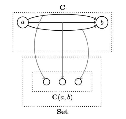
- It is possible, in some categories, to construct objects that represent hom-sets: internal hom-sets
9.1 - Univeral Construction
- Suspending belief that function types are sets momentarily, and try to construct an internal hom-set from scratch
- A function type may be considered a compositiee type because of its relation to the arguments and return type: thus we need a patteern which makes use of three objects representing function type, argument(s), and the return type
- This patteern is known as functional application or evaluation
- Given a candidate for:
- a function type ,
- an argument type ,
- the application maps this pair to
- We also have the application itself, which is a mapping
- Granularly, if we wanted to look inside these objects, we could select
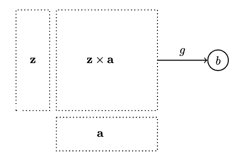
- But instead of dealing with individual pairs , we can deccribe the whole product of the function type and argument :
- is an object, and we can pick our application morphism, an arrow from that object to
- In , would be the function that maps every pair to
- This yields the desired patter: a product of two objects connected to another object by morphism :

- This pattern isn't specific enough to single out the function type using a universal construction for every category, but it works for the categories we're interested in at the moment
- Would it be possible to define a function object without first defining a product?
- There exist categories in which there is no product, or at least not a product for each pair of objects, so there's no function type if there's no product type
- Returning to universal construction, our imprecise query yields too many candidates, especially in the category of , where everything is connected to everything (excluding the empty set)
- Thus, we need to filter patterns by ranking like we've done in previously, eliminating candidates by requirements of:
- Unique mapping between candidate objects
- Mapping that factorizes our constructor
- We'll decree that , together with the morphism from is better than all other with their own if and only if there exists a unique mapping from such that the application of factors through the application of
- Thus, we need to filter patterns by ranking like we've done in previously, eliminating candidates by requirements of:

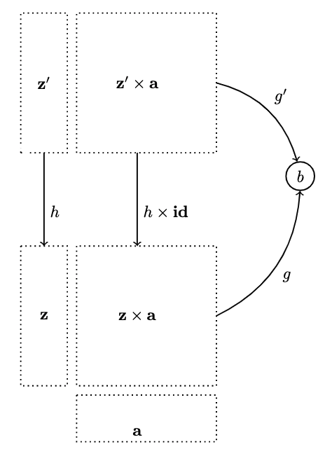
- Given , we want to choose the diagram that has both and crossed with ; that is, a mapping from . And we can do this because of the functoriality of the product
- I.e., we can lift pairs of morphisms, which is the definition not only of the product of objects, but also of morphisms:
- Since we're not touching the second component, the target of the morphism, we can lift with the morphism , where the latter component of the pair is an identity of
- We can factor one application out of another :
- Lastly, we must select the object which is universally besT which we'll call (a single object), which comes with its own application – a morphism from to – which we will call eval
- is the best if any other candidates for a function object can be uniquely mapped to it in such a way that its application morphism factorizes through eval

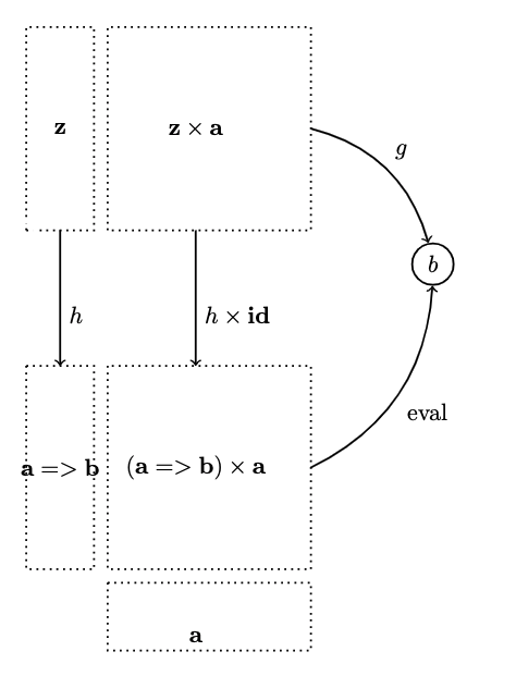
Formally:
- a function object from together with the morphism
such that, for any other object with a morphism
there is a unique morphism
that facotrs through
- There is no guarantee that object exists for any given pair of objects in a given category.
- It does happen to exist in , and then this object is also isomorphic to the hom-set
9.2 - Currying
- Take a look at all the candidates for the function object, this time considering the morphism as a function of two variables:
- Pretty much just a function of two variables. In Set, maps from pairs of values of two sets to another value in set
- The universal property tells us that for each , there exists a unique that maps to a function object :
- In Set, this just means that is a function of one variable type , and returns a function from to , making a higher order function
- Therefore, the universal construction establishes a one-to-one correspondence between a function of two variables and a function of one variable. This correspondence is called currying, and is called the curried version of
- The correspondence is one-to-one because, given any , there exists a unique , and given any , we can always recreate the second function using
- Currying is built into Haskell syntax:
a -> (b -> c)
a -> b -> c

-- trivial to convert between two representations with two higher order functions
curry :: ((a -> b) ->) -> (a -> b -> c)
curry f a b = f (a, b)

-- just the factorizer for the universal construction
uncurry :: (a -> b -> c) -> ((a -> b) ->)
uncurry f (a, b) =  f a b

-- where
f :: ((a, b) -> c) -> (a -> (b, c))
f g = \a -> (\b -> g (a, b))
9.3 - Exponentials
- The function object or the internal hom-object between two objects is called the exponential and denoted by
- It might appear weird at first that the argument type is in the exponential. Consider functions between finites types:
Bool,char,Int - Such functions can be fuly memoized and turned into lookup datastructures
- This is the essence of equivalence between functions which are morphisms and function types which are objects
- A pure function from Bool is completely specified by a pair of values corresponding to True/False
- The set of all possible functions from Bool to Int is the set of all pairs of Ints:
- It might appear weird at first that the argument type is in the exponential. Consider functions between finites types:
For example, C++'s char contains 256 possible values. Predicates like isUpper and isLower are implemented with lookup tables, equivalent to tuples of 256 boolean values. A tuple is a product, so the product of 256 bools is
- An iterated product defines a power, so we have read "bool to the power of char" =
9.4 - Cartesian Closed Categories
Cartesian Closed Categories must contain:
- The terminal object
- A product of any pair of objects
- An exponential for any pair of objects
- This category can be thought of as one supporting products of an arbitrary arity
- The terminal object can be though of as a product of zero objects or the zeroth power of an object
- A cartesian closed category that also supports the duals of the terminal object and product, and in which the product can be distributed over the coproduct:
is called a bicartesian closed category
9.5 - Exponentials and Algebraic Data Types
All the baseic identities of arithmeetic exponentials hold for these:
9.5.1 - Zeroth Power
Represents the set of morphisms going from the initial object to an arbitrary (Haskell's absurd Void -> a)
9.5.2 - Powers of One
Corresponds to the definition of the terminal object: there exists a unique morphism from any object to the terminal object which is the unit
9.5.3 - First Power
Corresponds to Haskell's () -> a, the isomorphism between elements of set , and the functions they that pick those elements
9.5.4 - Exponentials of Sums
States that the exponent from a coproduct of two objects is isomorphic to a product of two exponentials
9.5.5 - Exponentials of Exponentials
Expresses currying purely in terms of exponential objects: a function returning a function is equivalent to a function from a product (a two argument function)
9.5.6 - Exponentials over Products
A function returning a pair is equivalent to a pair of functions, each producing one element of the pair
9.6 - Curry-Howard Isomorphism
Just as:
Void, ()correspond to False, True respectively- Prod, Sum correspond to AND, OR
- correspond to "if a then b"
Curry-Howard Isomorphism states that every type can be interpreted as a morphism: T/F
- True if the type is inhabited, False otherwise
- I.e., logical implication is true if the function type corresponded to it is inhabited, which means that there exists a function of that type where the implementation of this function is itself a proof!
For example:
Which is modus ponens: if it's true that follows from , and is true, then must be true
Similarly, a false proposition cannot by implemented:
Either a b -> a
-- has no implementation sincee you can't product
-- a value of type a if you're called with the Right value
10 | Natural Transformations
I'm transcribing these chapters with a broken finger, so just infer any typos
We've esablished that a fuctor "embeds" one category within another, potentially collapsing multiple things into one, but never breaking connections
- Functors model one category within another
- There may be many different ways of embedding one category within another
- Natural Transformations help use compare different embeddings
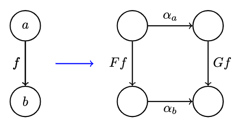
Consider two functors betweeen categories . If you focus on just one object , it is mapped to two object: . A mapping of functors should therefore map

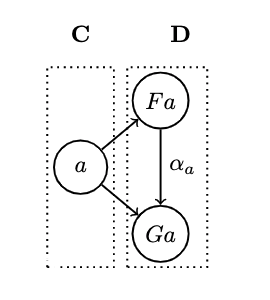
are objects in the same category , so mappings between them should conform to the same categories morphisms
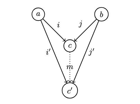
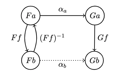
- A natural transformation is a selection of morphisms which, for every object , picks one morphisms from to . If we call the natural transformation , this morphism is called the component at :
Keep in mind that is an object in , and is a morphism in . If, for some , there is no morphism in , then there can be no natural transformation between
What about the morphisms mapped by functors? How do they fit into natural transformations?
- They're fixed: under any natural transformation between , must be transformed into . This constraint drastically reduces the number of choices we have in defining a natural transformation compatible with the desired mapping
Given a morphism between , it's mapped to two morphisms :
and the natural transformation provides tow additional morphisms that complete the diagram:

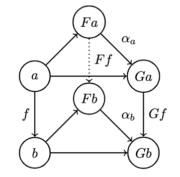
Now we have two ways of getting from . To ensure that they are equal, we impose that the naturality condition holds for any :
which is rather stringent: if morphisms is invertible, then naturality determines in terms of : it transports along :

- If there are more than one invertible morphisms between two objects, all these transportations have to agree.
- In general, morphisms aren ot invertible, so the existeence of a natural transformation between functors is far from guaranteed
- Component wise, natural transformations map objects to morphisms. Per the naturality condition, we can say that a natural transformation maps morphisms to commuting squares: there exists one commuting naturality square in for all morphisms in

- Natural transformations may be used to define isomorphisms of functors:
- Two functors which are naturally isomorphic are "basically the same"
- A natural isomorphisms is defined as a natural transformation whose components are all isomorphisms (or invertible isomorphisms)
10.1 - Polymorphic Functions
- To construct a natrual transformation, we start with an object: type
a- One functor
Fmaps it to the typeFa - And another functor
Gmaps it to typeGa - The component of thee natural transformation at is a function from
Fa -> Ga - It's polymorphic on all types
a
- One functor
alpha :: forall a . Fa -> Ga
-- `forall` is an optional Haskell language extension
It's a family of functions parameterized by
a- In Haskell, a polymorphic function must be defined uniformly for all types: parametric polymorphism
- In bad languages (c++) templates don't have to be well defined, instead being chosen at instantiation-time: ad hoc polymorphism
Haskell's parametric polymorphism has the consequence that any polymorphic function of type
alpha :: Fa -> Ga
where F, G are functors automatically satisfies the naturality condition:
- The action of the functor
Gon morphismfis implemented usingfmap:
fmap_G :: . alpha_a = alpha_b . fmap_F f
-- pseudo explicit type annotations, but the following works via compiled

fmap f . alpha = alpha . fmap f
- Because of the stringency of parametric polymorphism, we get satisfaction of the naturality condition for "free"
- If functors are containers, natrual transformations are recipes for repackaging contents of one container into another
- The naturality condition becomes the statement that it doesn't matter if we modify the items first, and then repackage, or repackage and theen modify; the two actions are orthogonal
For example: A natural transformation between the List functor and Maybe functor, returning the head of the list if it's non-empty:
safe_head :: [a] -> Maybe a
safe_head [] = Nothing
safe_head (x:xs) = Just x
this function is polymorphic in a for all a! Therefore it is also a natural tranformation between the two functors.
We can verify as well:
fmap f . safe_head = safe_head . fmap f
-- 2 cases:
-- case 1: empty list

fmap f (safe_head []) = fmap f Nothing = Nothing
safe_head (fmap f []) = safe_head [] = Nothing

-- case 2: non-empty
fmap f (safe_head (x:xs)) = fmap f (Just x) = Just (f x)
safe_head (fmap f (x:xs)) = safe_head (f x: fmap xs) = Just (f x)
- When one of the functors is the trivial
Constfunctor, the natural transofmration to or from it looks just like a function that's either polymorphic in its return type or argument type, i.e.lengthas a natural transformation fromListtoConst Int:
length :: [a] -> Const Int
length [] = Const 0
length (x:xs) = Const (1 + unConst (length xs))

-- where

unConst :: Const c a -> c
unConst (Const x) = x
- Finding a parametrically polymorphic function from a
Constfunctor is harder since it requires creation of a value from nothing- The best we can do is something like:
scam :: Const Int a -> Maybe a
scam (Const x) = Nothing
- Another common functor is the
Reader
newtype Reader e a = Reader (e -> a)
-- parameterized by two types, but is covariantly functorial only in the second
  fmap f (Reader g) = Reader (\x -> f (g x))
For every type e, we can define a family of natural transformations from Reader e to any other functor f:
- I.e., the unique type with one element
(), the functorReader ()takes any typeaand maps it into a single function type() -> awhich is all the functions that pick a single element from the seta, of which there are as many as there are elements ina - Consider a natural transformation to the
Maybefunctor:
alpha :: Reader () a -> Maybe a
-- just 2
dumb (Reader _) = Nothing
obvious (Reader g) = Just (g ())
10.2 - Beyond Naturality
- A parametrically polymorphic function between two functors (including the oddity fof the
Constfunctor) is always a natural transformation since all standard ADTs are functors, any polymorphic function between those types is a natural transformation - We can also use function types, which are functorial in their return type, to build functors and define natural transformations that are higher order functions
- Not covariant in argument type, but are contravariant
- Recall that this implies that they're equivalent to covariant functors from the opposite category
- Therefore, polymorphic functions between two contravariant functors are still natural transofrmations in the categorical sense, just working on functors from the opposite category
For example, the familiar contravariant functor:
newtype Op r a = Op (a -> r) -- is contravariant in `a` by

instance contravariant (Op r) where
  contramap f (Op g) = Op (g . f)

-- allowing us to write a polymorphic function from Op -> Bool, Op -> String, etc
predToStr (Op f) = Op (\x if f x then "T" else "F")
But since the two functors are not covariant, this is not a natural transformation in Hask, but since they're both contravariant, they satisfy the "opposite" naturality condition
contrampa f . predToStr = predToStr . contramap f

-- note that f must go in the opposite dir to than what we'd use
-- with fmap bc of the signature of contramap :

contramap :: (b -> a) -> (Op Bool a -> Op Bool b)
What about type constructors that are not functor, like a -> a?
- This is not a functor since the same type
ais used in both the positive covariant and negative contravariant position - Therefore, we can't implement
fmaporcontramapfor this type
(a -> a) -> f a
-- can't be a N.T., but dinatural transformations, a generalization of
-- this pattern, let us deal with such cases
10.3 - Functor Category
- Since we can map between functors via natural transformations, do functors constitute a category? yeeaa boi
- For each pair of categories , there exists a category where
- objects are functors from
- morphisms are natural transformations beetween these functors
- To define a composition of natural transformations, we simply look at the components of the natural transformations which themselves are composable morphisms
For example, take the natural transformation from to whose component at is some morphism
and we want to compose with which is another natural transformation from to with the component at given by
These morphisms are composable as follows:
which can be the component of the natural transformation , the composition of two natural transformation "β after α":

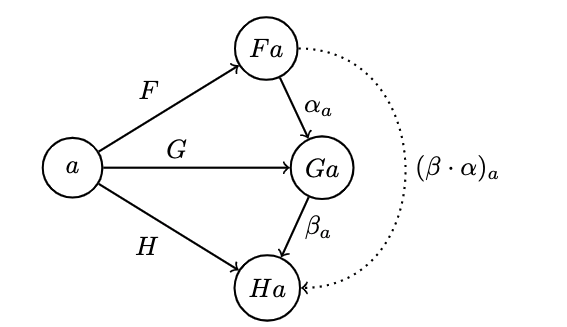
Which expresses that the resultant composition is a natural transformation from :

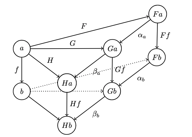
- Composition of natural transformations is associative because they are components, which are regular morphisms, which are associative with respect to composition
- For each functor , there exists an identitive natural transformation whose components are the identity morphisms
Therefore, functors form a category.
Noational Aside About "" vs ""
- Dot notation is preferred for this kind of natural transformation, but know that there are two ways of composing them: vertically, and horizontally
The diagrams above utilize the former whereas the following diagram uses the latter:

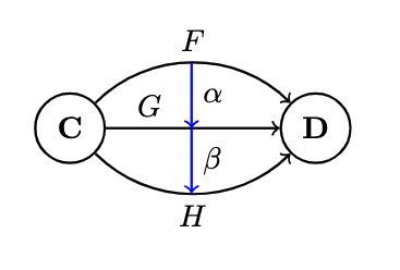
The functor category between categories is written , or , or where the last expression indicates that a functor category itself might be considered a function object (an exponential) in some other category since an object in a product category consists of a pair of object , a morphism between two such pairs is a pair of morphisms where
which compose component wise – and we know that there's always an identity pair.
Thereform, is a cartesian closed category in which there exists an exponential object (a category!) for any pair of categories which is just the functo category between
10.4 - 2-Categories
- By definition, any hom-set in Cat is a set of functors (with richer structure than just a set) which form a category with natural transofmration acting as morphisms (morphisms between morphisms)
- This richer structure is an example of a 2-cateogry: a generalization of a category where, besides objects and morphisms (which might be called 1-morphisms in this context), there are also 2-morphisms, which are those between morphisms
Cat as a 2-category:
- Objects: small categories
- 1-morphisms: functors between categories
- 2-morphisms: natural transformation between functors
Instead of a hom-set between two categories , we have a hom-category . We have a regular functor composition: functor from composed with functor from to yield from
But we also have composition within each hom-category – vertical composition of natural transformations (2-morphisms between functions)
How do these two types of composition interact? Take two functors (1-morphisms) in Cat:
and their composition
and suppose we have two natural transformations acting on respectively

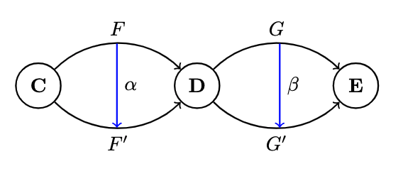
Note that we can't apply vertical composition to this pair because the target of is different from the source of
- We can, however, apply composition to since the target of the former is the source of the latter:
- What's the relation whetween and ? With at our disposal, we can define a natural transformation from :

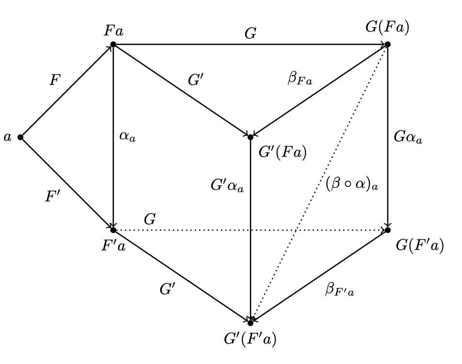
Let's break that one down:
- Starting with , its image splits into two object in which are connected by the morphism, a component of :
- When going from , these two object split further into four objects:
- with four morphisms forming a square, two of which are the components of the natural transformation :
and the other two being symmetric images of under the two functors:
- We want a morphism which goes from , a candidate for the component of a natural transformation connecting the two functors
and there are two such paths we can take from :
which are equal because the square we formed happens to be the naturality square for
- We've defined a component of a natural transformation from . We call it the horizontal component of :
A good rule of thumb is that: every timee we encounter a composition, look for a cateegory.
- With vertical composition, which is a part of the functor category
- Whatabout the horizontal composition then? Where does that live?
Consider Cat sideways, where the natrual transformations are not arrows between functors, but as arrows between other categories. A natural transformation sit between two categories, the ones connect by the functors it transforms:

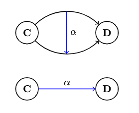
- If we focus on two objects of Cat , we can observe a set of natural natural transformation that go between functors connecting them ().
- These natural transformation are our new arrows from . Similarly, there are natural transformation from , which we can treat as arrows from and to, respectively.
- Horizontal composition is the composition of these arrows
- We also have the identity arrow from to itself, which is just the identitive natural transformations that maps the identitive functor on to itself
- Not that the identitive horizontal composition is also the identity for vertical composition, but not vice versa
- Finally, the two compositions satisfy the interchangeability law:
- In this sideways interpretation of Cat, there are two ways of getting from object to object: a functor, or a natural transformation
- We can re-interpret the functor arrow as a special kind of natural transformation: the identitive natural transformation acting on this functor: where , and is the natural transformation from
- Since we can't compose a functor with a natural transformation, this should be interpreted as a horizontal composition of the identity natural transformation after . Similarly, is a horizontal composition of after
10.5 - Conclusion
- This concludes the first section, covering "basic" vocabulary and grammar of category theory:
- Objects: nouns
- Arrows:
- Morphisms: connect objects
- Functors: connect categories
- Natural transformation: connect functors
Abstraction
- A set of morphisms becomes a function object which can be the source or target of another morphism, resulting in higher order functions
- A functor maps objects to objects, so we can use it as a type constructor or a parametric type. They can also map morphisms, so they're like higher order functions like
fmap- Simple functors include
Const, product, and sum which can be used to build more complex data types - Function types are also functorial, both covariant and contravariant
- Simple functors include
- Functors are objects in the functor category, acting as the source and target of morphisms (natural transformation) - which themselves are special polymorphic functions
11 | Declarative Programming
Composition may be defined declaratively:
h = g .f
or imperatively: call f, store the result, call g on result:
h x = let y = f x
      in g y
which is more sequentially-coded. I.e., g cannot happen beforee the eexecution of f completes (at least, that's the interpretation in a lazy, call-by-need language) - but the compiler might do some clever inlining/wizardy to blur the lines between the two methodologies
- The two methodologies differ drastically, begging the question: do we always have a choice, and if a declarative solution exists, can it always be translated into code? The answer is nebulous
11.1 - Physics Anecdote
In physics there's a duality of expressing laws
- First: using local or infinitesmal considerations by examining a system under a microlens and predicting how it will evolve within the next instant of time
- This frame of understanding usually expresses systems in terms of differential equations to be integrated over a time interval, which resembles imperative thinking: a solution can be reached by following a sequence of smaller steps which are dependent on the previous step
- E.g., a game of asteroids may be modeled by iterating over a set of differential equation:
and this trival example can be extended to more complex systems and underlying process of discretzing time and space
- The other approach is global, examining instead initial and final system states and computing a "trajectory" connecting them by optimizing a certain function, i.e. Fermat's principle of Least Time which states that
Light rays propagate along paths ftat minimize flight time (in the absence of reflecting or refracting objects, this is a straight line). The path of minimal time makes the ray refract at the boundary of meterials with different densities, yielding Snell's law
where are the velocities of light in the different materials, and are the angles from the normal to the boundary.
- All of classical mechanics can be derived from this pronciple of Least Action which be calculated for any trajectory by integrating the lagrangian which is the difference (as the sum would be the total energy) between the kinetic and potential energies of the states.
- Feynman generalized this principle to quantum mechanics, formulating the problem in terms of initial and final states. A Feynman Path integral between initial and final states is used to calculate the probability of transition between states
- The point of all this being that there exists a duality in the way we can describe things, with the main difference being the way that we treat or represent time
- Category Theory encourages the latter, global approach which aligns with declarative programming
- In category theory, there is no notion of distance, neighborhoods, or time; just abstract objects and abstract connections between them
- If you can get from to in a series of steps, you can also get there in one step (the composition of hte constituent steps)
- The universal construction also epitomizes the global approach
12 | Limits and Colimits
- Revisiting the universal construction of the product, let's see if we can't simplify and further generalize it with our new knowledge of functors and natual transformation
- Recall that the construction of a product starts with the selection of two objects . What does it mean to select object?
- We can abstract this into more "categorical" terms by considering a category called with just two objects in it: , and no morphisms other than the obligatory identities
- Now, selection of two objects in can be rephrased as the definition of a functor from , mapping the two objects to their images (or image if the functor collapses, which is fine) as well as the identity morphisms in to
- This construction removes the imprecise terms of "selection" and replaces it with well defined categorical directive

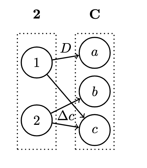
- Now, to "select" the candidate object , we use the constant functor from by which maps all objects into and all morphisms into
- Now, with two functors from we can consider possible natural transformations between them. We have two componenets:
- object mapped to by and to by , so the component of a natural transformation between , at is a morphism from call it
- The second component is a morphisms , the image of object under
- These directly correspond to the two projections used in the original construction of a product. Instead of selecting an object and projections, we instead use functors and natural transformations
- And, because in our trivial example, there are no morphisms in other than the identity, the natural condition is satisfied!

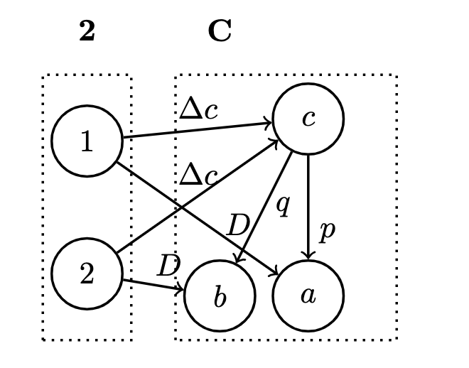
Further generalizations which contain non-trivial morphisms will impose natural conditions on the transformation between and
- We call such transformations a cone where the image of is the apex of a pyramid whose sides are formed by the components of the natural transformation, and forms the base
To build a cone, we start with a category that defines the pattern, usually a small, finite category
- Pick a functor from and call its image a diagram
- Pick some as the apex and use it to define the constant functor from
- A natural transformation from is the cone
For finite , it's just a bunch of morphisms connecting to the diagram, that is: the image of under
- naturality requires that all triangles (walls of a cone) in this diagram commute
- Take any morphism in , not that maps it to a morphism , a morphism that forms the base of some triangle
- The constant functor maps to the identity morphism on and squishes the two ends of the morphism into one object, and thus the naturality square becomes a commuting triangle, two arms of which are the components of the natural transformation
Nother cone
- This constructs one cone, but we want a universal cone, and there are many possible ways to do this
- We can define a category of cones based on a given functor where objects are cones, but not every object can be an apex of a cone since there might not be a natural transformation from
- We also need morphisms between cones which would be etermined by morphisms between cone apexes, but we've added the constraint that morphisms between candidate objects must be common factors for the projections
p' = p . m
q' = q . m
which translates, in the general case, to the condition that the triangle whose one side is the facotrizing morphism all commute
[image of such a N.T.]
The bold lines of such an image of such a natural transformation represent the commuting triangle connecting two cones, with teh morphism (the lower cone being the universal one, with ) is its apex.
- Take those factorizing morphisms as the morphisms in our category of cones, and we can easily verify the conclusion that they compose, and are identitive. Therefore, cones form a category
Now, we can define the universal cone as the terminal object in the category of cones, there is a unique morphism from any object to that object
- In this case, there must be a unique, factorizing morphism from the apex of any other cone to the apex of the universal cone
- We call this universal cone the Limit of the diagram
- As shorthand, the apex of this cone ca be called the limit since the apexes are our primary "handles" on the cones in this category
The limit embodies the properties of the whole diagram in a single object. For example, the limit of the two-object diagram in the above is the product of the two objects. The product together with the two projections contains the information about both objects with no extraneous junk, thus making it universal