Towards Computational Game Theory Part 2
- Published on
- ∘ 16 min read ∘ ––– views
Tags
Previous Article
Next Article
Preface
This post builds on my previous installment on Game Theory, exploring more complex games and the ways that they're modeled which I found to be interesting.
It started off as an exercise in implementing a generic Monte Carlo Tree Search algorithm which could solve simple 2-player board games such as Tic Tac Toe and Connect Four. There already exist numerous articles about implementing this algorithm, and my deviations from them adds little value other than "ooh, looky, a generalized abstract representation of a Game." After hacking together some gross code which managed to consistently win or tie myself and itself respectively, I started to search for other games which would be appropriate for my rinky dink MCTS.
The Game interface I had designed was well-suited for 2-dimensional board games which take place on a rectangular grid (though my "research" also indicated that it could be easily? extended to other board representations like a hexagonal grid1). The natural successor for the games I had already implemented was Chess, but I was also aware that my scuffed implementation would likely buckle under the magnitude of the search space of Chess.
One of my friends suggested the game of Dots and Boxes -the trivial children's game– and that's when I went down the rabbit hole.
Dots and Boxes: Building the 4th Wall
If you've never had the pleasure of occupying yourself and a sibling while waiting for a delayed flight, or perhaps on a long car trip before you were old enough to be infected by electronics, you might not have played this game. It's very simple:
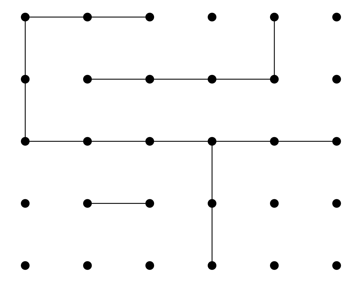
- The board consists of a grid of dots
- Players take turns connecting two adjacent dots
- The player who closes a square fills it with his token (be it his initials, or grotesque depiction of his opponent) and gets to draw another edge until he fails to complete a square
- This sequence continues until all possible edges are filled out, and the player who completed the most squares is declared the winner
- The loser then is unceremoniously taunted for their inability to complete squares as intelligently as the victor, and then usually the two contestants are warned that if they don't stop arguing, a can of whoopass will be dispatched upon them

Simple enough, right? -the trivial children's game–.
No. In fact, it turns out that consistently winning this game is not so simple. There are multiple tiers of intermediate 2 and high level strategy, as well as an entire field of mathematics dedicated to the study of such games known as Combinatorial Game Theory. Turns out the solution is is not trivial and optimal play is actually very difficult to achieve as we'll see shortly.
Combinatorial Game Theory
Much of what follows is an amalgamation of wikipedia articles, books, and publications about this field. This section is supposed to be a concise ( ¯\(ツ)/¯ ) summary of the relevant bits as they pertain to winning Dots and Boxes.
A common model of a game within Combinatorial Game Theory consists of a set of possible moves that the players can make at any given state of play. For the sake of simplicity, I'll confine discussion to 2-player games like those mentioned above. The two players are referred to as and . A game is then represented as
Where either partition of the game is the set of moves that each player can take.
Domineering
Another 2-player combinatorial game which fits this model is known as Domineering. Also taking place on a grid, this game pits players Left (horizontal) and Right (vertical) against one another in an effort to fill the grid with their domino-shaped tiles. A player wins when their opponent is unable to make a move:

Here, the blue horizontal player wins the game since red vertical player is unable to make a move at the start of the 7th turn (move 13).
At turn 0, a generic game of Domineering is represented as
Subsets of the whole game state can be examined and represented using Nimbers – a notation used to describe how many moves each player has remaining for any given game state.
For example, given the following board:

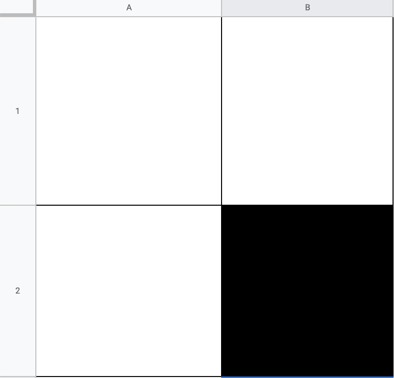
The game is expressed as
This results in the zero-game: in which there is only one remaining move for either player, and if either player takes that move, they will win having left their opponent with no remaining moves
- Note that whose turn it is is implicitly encoded in the game state
Numbers and Nimbers
Nimbers describe unique positions in finite, impartial games. Their name is derived from the game of Nim, where players draw objects from heaps attempting to force the other player to take the last object. The game indicates the number of free or legal moves for each player. In most combinatorial games like Domineering, or Dots and Boxes, left and right values are an approximation of advantage. Positive numbers indicate an advantage for the Left player, and negative for the Right.
Nimbers are defined recursively from the following base cases:
Other named or notable states of play include:
- The star-game: ; in which the 1st player to move wins the game since she moves from it () to the zero-game in which the opponent has no valid moves.
- Up, : ;
- Down, : ;
- A hot-game, : is a state where both players desire to move, as both moves provide an advantage to the player that takes one.
- A game is said to be hot if
And "fuzzy" for all in between.
(Inexhaustive) Properties of Nimbers
- Nimbers can be summed as integers: :)
- Hot games can be added and multiplied with positive numbers:
- Nimber addition can be used to calculate the size of a single nim-heap equivalent to a collection of heaps:
where is the minimum-excludant operation on a set of ordinals defined to be the smallest ordinal that is not an element of the set. For finite ordinals, the Nim-sum is evaluated via the bitwise XOR: . Not to be confused with finite orders of dim sum which are evaluated via how yummy it is.

- Building off of addition, Nimber multiplication is defined as
These two properties together form a proper class determining an algebraically closed field of characteristic 2 with additive and multiplicative identities:
Sprague-Grundy Theorem
So why do we need Nimbers? They help use to describe game states that can pop up across several types of combinatorial games.
According to the Sprague-Grundy Theorem, every partial game under normal play convention is equivalent to a one-heap game of Nim.
Every game, then, can be expressed as a natural number, the size of the heap in its equivalent game of Nim, as an ordinal in the infinite generalization, or as a Nimber: the value of that one-heap in an algebraic system whose addition operations combines multiple heaps to form a single equivalent heap in Nim.
The Grundy Value (Nimber) of a game is the unique number that the game state is equivalent to. The theorem assumes that a game is a 2-player, sequential game of perfect information which is guaranteed to terminate under normal play conditions – that is, a player who cannot move loses.
- A Partial game is one in which and might have different move sets on the same board (e.g., horizontal and vertical in the case of Domineering)
- An Impartial game is one where both players have identical move sets for each state (e.g., Nim, Tic-Tac-Toe)
Formally, we define Grundy values as follows:
Every finite, impartial game has a single value according to the theorem, and these impartial games can be combined via Nim-addition:
Properties of Grundy Values
- Positions in impartial games fall into two outcome classes:
- Either the next player to move wins: -position
- Or the previous player wins: -position
For example: is a -position, while is an -position.
We say that two games are equivalent if, no matter what position is added to them, they always have the same outcome. That is, is in the same outcome class as .
Nim Trace with Grundy Values
Here, A, B, and C are the heaps in an instance of Nim:
| Turn | A | B | C | Move | Position |
|---|---|---|---|---|---|
| 0 | 2 | 2 | 2 | initial game state | |
| 1 | 1 | 2 | 2 | Alice takes 1 from A | |
| 2 | 0 | 2 | 2 | Bob takes 1 from B | |
| 3 | 0 | 1 | 2 | Alice takes 1 from C | Alice has three options: remove 2 from C, 1 from C, or 1 from B. Removing 2 from C leaves Bob in position Removing 1 from C leaves bob with two piles of heap size 1: Removing 1 from B leaves bob with two objects in a single pile s.t. his moves would be , so Alice's move would result in position The set of all her moves is then |
| 4 | 0 | 1 | 1 | Bob takes 1 from B | his moves are identical insofar as they leave Alice in the same position (thus he has one move: ) |
| 5 | 0 | 0 | 1 | Alice takes 1 from C | since her move leaves Bob in position |
| 6 | 0 | 0 | 0 | Bob has no moves, fuckin loser 🤪 |
Dots and Boxes Revisited
So yeah, it turns out that there's a lot more at play here than meets the eye, and according to Berlekamp, Conway, and Guy in Winning Ways for Your Mathematical Plays 3 as well as Demaine and Hearn,4 determining the winner of a sufficiently large game of dots and boxes is NP-hard.
I've included the proof construction because its funny:
Winning Ways argues that Strings-and-Coins (the dual of Dots and Boxes) is NP-hard as follows. Suppose that you have gathered several coins but your opponent gains control. Now you are forced to lose the Nimstring game, but given your initial lead, you still may win the Strings-and-Coins game. Minimizing the number of coins lost while your opponent maintains control is equivalent to finding the maximum number of vertex-disjoint cycles in the graph, basically because the equivalent of a double-deal to maintain control once an (isolated) cycle is opened results in forfeiting four squares instead of two [duh lol]. We observe that by making the difference between the initial lead and the forfeited coins very small (either or ), the opponent also cannot win by yielding control. Because the cycle-packing† problem is NP-hard on general graphs, determining the outcome of such string-and-coins endgames is NP-hard. Eppstein observes that this reduction should also apply to endgame instances of Dots-and-Boxes by restricting to maximum-degree-three planar graphs. Embedability of such graphs in the square grid follows because long chains and cycles (longer than two edges for chains and three edges for cycles) can be replaced by even longer chains or cycles.
It remains open whether Dots-and-Boxes or Strings-and-Coins are in NP or PSPACE-complete from an arbitrary configuration. Even the case of a grid of boxes is not fully understood from a Combinatorial Game Theory perspective.
† - The Cycle Packing problem asks whether an undirected graph contains vertex-disjoint cycles. It's implied that Strings-and-Coins can be reduced to an instance of this problem, and that this reduction holds for the dual of Strings-and-Coins which is Dots-and-Boxes.
Nevertheless, we can use the Sprague-Grundy theorem to statically analyze smaller boards (rather than stochastically via a Monte Carlo simulation, as I initially set out to do). Note that this static analysis is still NP-hard, but at least it's more tractable for reasonably sized boards.
An unreasonably sized board is one whose duration of completion spans more than one layover at an airport.
Static Analysis Example
Let's take a look at an example from Berlekamp's book mentioned in the proof construction above.
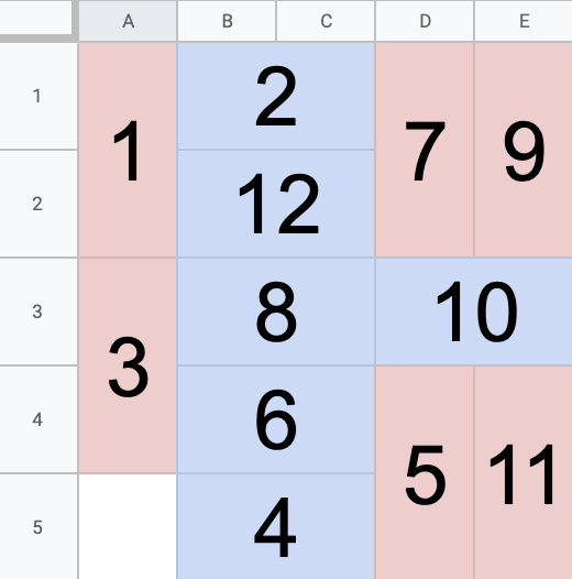
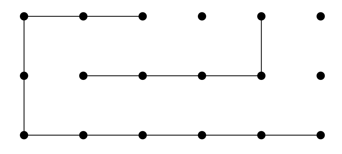
Given the following instance of Dots-and-Boxes, there are 33 possible moves (horizontal and vertical edges yet to be drawn between dots).

The game will likely have a score or more turns, which would be catastrophic for my laptop's memory were I to try to simulate play on this relatively small board. (The game of Connect Four dodges this search space issue by way of forced dimension reduction: players can only select which column to play in, the row space shrinks as a byproduct of columnal play).
The game state can be divided into 3 positions with corresponding Nimbers which can be dynamically computed in time (exponential in the number of remaining moves):
 |
 |
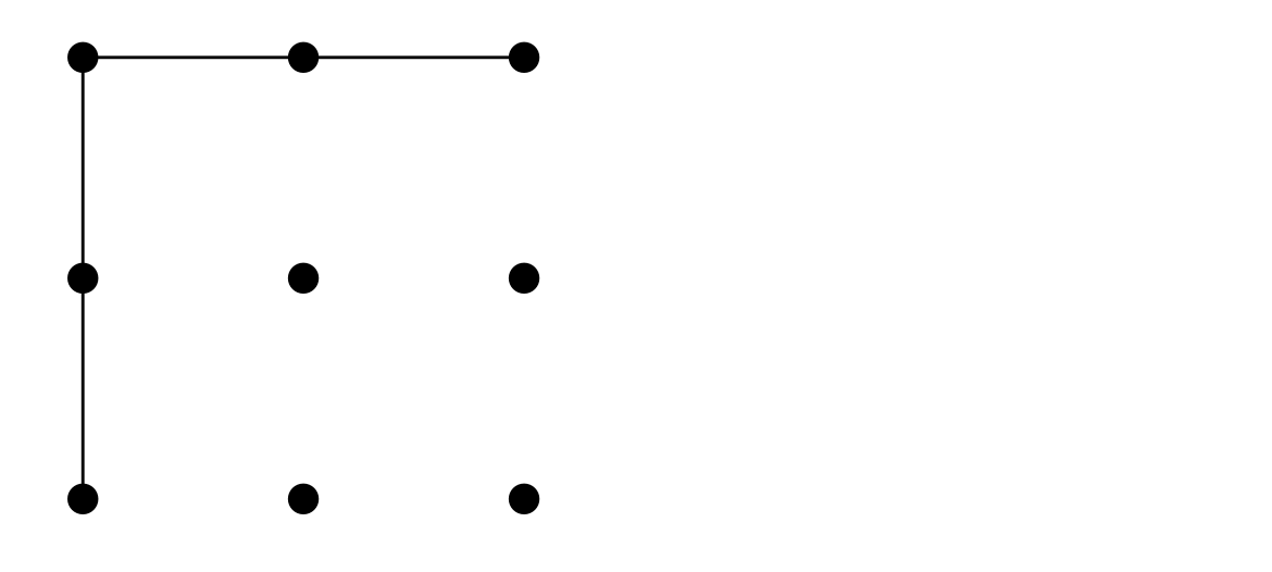 |
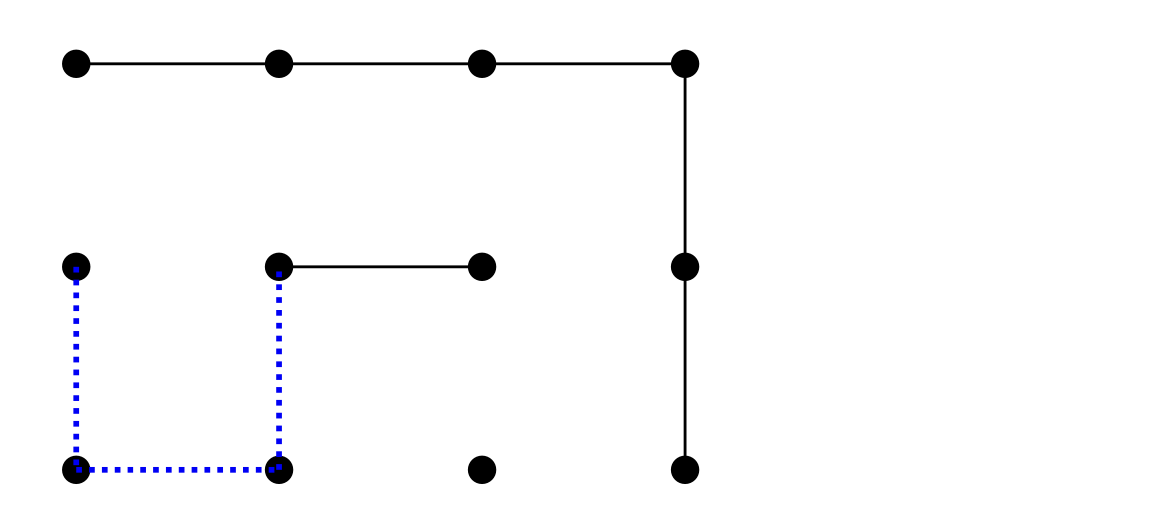
Recall that we can generalize winning the combinatorial game we are playing to the goal of leaving our sibling adversary in the zero position from whence he hath no moves!
Adding the Nimbers via the XOR operation, we get :
but we want this to sum to , so we play a move on one of the positions which will cause this result. The only winning move for this configuration is to change to by any of the dotted blue edges in , yielding the following bitwise Nim-sum:
The only missing pieces of the puzzle are a board decomposition algorithm and dynamic programming computation of Nimbers for board positions. Not small feats by any means, but what's a rainy day without a backlog of projects to work on!
Further Reading
Romer, Abel. "Winning Dots-and-Boxes in Two and Three Dimensions." Quest Unversity Canada.
Barker, Joseph and Richard Korf. "Solving Dots-and-Boxes." AAAI.
References
Footnotes
Moghadam, Masoud M. "Monte Carlo Tree Search: Implementing Reinforcement Learning in Real-Time Game Player | Part 3." Towards Data Science. ↩
Numberphile. "How to always win at Dots and Boxes - Numberphile." YouTube. ↩
Berlekamp, Elwyn R. et al. "Winning Ways for Your Mathematical Plays: Volume 1 (AK Peters/CRC Recreational Mathematics Series)." do you really care who published it?. ↩
Demain, Erik and Robert Hearn. "Playing Games with Algorithms: Algorithmic Combinatorial Game Theory∗." MIT, I think? ↩