Towards Computational Game Theory Part 1
- Published on
- ∘ 33 min read ∘ ––– views
Tags
Previous Article
Next Article
Preface
The front half of this post is mostly explanation, and the latter half are notes.
Contents
- Preface
- Contents
- Intro to Game Theory: a Lightspeed Overture
- Types of Games
- Types of Agents
- Formalizing Game Theory
- Linear Programs
- The Lagrangian
- Further Reading
Intro to Game Theory: a Lightspeed Overture
Broadly speaking, Game Theory is a field dedicated to modeling the interactions between different (types of) agents, and it has vast applications. As the section header indicates, this is a super crash course, but I highly recommend doing some further reading because this topic is SO COOL.
You know the drill: first, some definitions.
Glossary
- Agent: A player in a game
- Game: Usual represented as a payout matrix (or tensor, or a graph for games with multiple players). Types of games include:
- Zero Sum: One player wins at the expense of all others – purely competitive. Examples include: poker, chess, checkers, (most conquest-driven board games), cake cutting (divided unequally). Formally, if we have then, in a zero-sum game: .
- Non-zero Sum: One player's strategy does not necessarily impact the outcome for another player. These games can be win-win. Examples include: Battle of the Sexes, Prisoner's Dilemma, markets.
- Constant-Sum: one where there exists some constant such that, for each strategy profile . It's like a zero-sum game, but replace 0 with .
- General Sum: In these games, there is no optimal strategy, instead players choose the best response to their opponent's strategy.
An example of a generic "game" might look like this:
B | ||
|---|---|---|
A | 2, 4 | 0, 2 |
10, 2 | 2, 0 | |
An additional note to make is that agents in different types of games can have imperfect information as well as incomplete information.
Incomplete Information means there are things you simply don't know, such as the opponent's strategies or payoffs. Imperfect Information means you won't know when or if an opponent makes a move.
- Strategy: Set of rules an agent follows in order to maximize the utility of their outcome
- Dominant: Exists in a game where there is a single optimal strategy for each player, regardless of what their opponent(s) choose. In the above example, player A has a dominant strategy since, regardless of what player B chooses, their optimal outcome is to play down-left.
- Pure: A pure strategy is one where the agent chooses an action consistently.
- Mixed: A mixed strategy is one where a player chooses a strategy based on a probability distribution over strategies available to her.
- Nash Equilibrium/Equilibria: A set of strategies over players are said to be at Nash Equilibrium if all players' optimal choices coincide with one another such that neither player/no players would want to change their behavior or strategy after other players' strategies are revealed. This implies that players choose the optimal strategy according to what they assume other rational players will select for their respective strategies.
- There can be multiple Nash Equilibria in a given game, for example:
B | ||
|---|---|---|
A | 1, 1 | -1, -1 |
| -1, -1 | 1, 1 | |
For games with mixed strategies at play, the equilibria are determined by the optimal frequency of when to play a certain strategy given consideration of other players' distributions.
In general, games can have one of the four types of Nash Equilibria:
- Only one pure Nash Equilibrium (e.g. in Prisoner’s Dilemma)
- Only one mixed Nash Equilibrium and no pure Nash Equilibrium (e.g. Kicker/Goalie Penalty kicks)
- At least one player picks a "random" strategy such that no other player is able to increase her expected utility by playing an alternate strategy
- Multiple pure Nash Equilibrium (e.g. Chicken)
- Pure and mixed (e.g. Chicken)
What the hell are are these games?? Thanks for asking.
Types of Games
There are numerous examples of 2 player games:
1. Prisoner's Dilemma (one shot)
Perhaps the most quintessential "game." Guy de Maupassant provides an excellent depiction of this game in his short story Two Friends. Consider the following excerpt:
The two fishermen remained silent. The German turned and gave an order in his own language. Then he moved his chair a little way off, that he might not be so near the prisoners, and a dozen men stepped forward, rifle in hand, and took up a position, twenty paces off.
"I give you one minute," said the officer; "not a second longer."
Then he rose quickly, went over to the two Frenchmen, took Morissot by the arm, led him a short distance off, and said in a low voice:
"Quick! the password! Your friend will know nothing. I will pretend to relent."
Morissot answered not a word.
Then the Prussian took Monsieur Sauvage aside in like manner, and made him the same proposal.
Monsieur Sauvage made no reply.
Again they stood side by side.
The officer issued his orders; the soldiers raised their rifles.
Then by chance Morissot's eyes fell on the bag full of gudgeon lying in the grass a few feet from him.
A ray of sunlight made the still quivering fish glisten like silver. And Morissot's heart sank. Despite his efforts at self-control his eyes filled with tears.
"Good-by, Monsieur Sauvage," he faltered.
"Good-by, Monsieur Morissot," replied Sauvage.
They shook hands, trembling from head to foot with a dread beyond their mastery.
The officer cried:
"Fire!"
The twelve shots were as one.
B | |||
|---|---|---|---|
confess | silence | ||
A | confess | -1, -1 | -4, 0 |
| silence | 0, -4 | -3, -3 | |
Here, the two Frenchman poetically, but irrationally chose to remain silent. Here, the numbers chosen are sort of arbitrary; any game with payouts following this relation can be considered an instance of the Prisoner's Dilemma:
B | |||
|---|---|---|---|
cooperate | defect | ||
A | cooperate | a, a | b, c |
| defect | c, b | d, d | |
2. Battle of the Sexes
The Battles of the Sexes is a coordination game between a couple who can't agree on how to spend their evening together. The wife would like to go to a ballet, and the husband a boxing match. Each would rather spend their time together at the activity they least prefer rather than spend the evening on their lonesome at their preferential activity:
Husband | |||
|---|---|---|---|
boxing | ballet | ||
Wife | boxing | 3, 2 | 0, 0 |
| ballet | 0, 0 | 2, 3 | |
3. Chicken
Chicken is an example of a pure coordination game as the agents have no conflicting interests. Consider two vehicles speeding towards each other. They must mutually, but independently of one another (i.e., without communicating), decide which direction to swerve –or, less violently, which lane to drive in– so as not to hit the other player. Pray that you're not playing against a Brit!
Left | Right | |
|---|---|---|
Left | +1, +1 | 0, 0 |
Right | 0, 0 | +1, +1 |
4. Rock, Paper, Scissors
Need I explain the rules? Now we introduce a more interesting "game" model:
Rock | Paper | Scissors | |
|---|---|---|---|
Rock | 0, 0 | -1, +1 | +1, -1 |
Paper | +1, -1 | 0, 0 | -1, +1 |
Scissors | -1, +1 | +1, -1 | 0, 0 |
What are the Nash Equilibria for Rock, Paper Scissors, if any? This game falls under the second category of Nash Equilibria: one with only 1 mixed Nash Equilibria and no pure strategy. If a player attempted to employ a pure strategy, i.e., always pick rock, then they would easily be exploited by any other player by simply choosing paper. So how, then, do we compute the equilibria? Say we have players with respective (identical) utility functions according to the above payout matrix where is the probability that plays rock, etc. If we enumerate the expected value of each respective option available to them:
Then we can conclude that
On the real, the best way to win at RPS is to wait like half a second for your opponent to throw their selection, then throw its usurping strategy and gaslight your opponent until they concede.
5. Penny Matching
Penny Matching is another example of a zero-sum game. The premise is that there are two players, Even and Odd. The goal for the Even player is to match the Odd player's selection, and the goal for the Odd player is the inverse: to be an utter deviant, a copper crook, a parsimonious penny pilferer, a fractional filcher.
Even | |||
|---|---|---|---|
Heads | Tail | ||
Odd | Heads | +1, -1 | -1, +1 |
| Tails | -1, +1 | +1, -1 | |
This is another example of a mixed strategy game. Consider what happens if we modify the payouts like so:
Odd | |||
|---|---|---|---|
Heads | Tail | ||
Even | Heads | +5, -1 | -1, +1 |
| Tails | -1, +1 | +1, -1 | |
It would appear to behoove the Even player to try to play Heads as much as possible, but Odd knows this as well. Enter the spiral of inductive reverse psychology! Or, simply compute the Expected Utility for each player to determine at what frequency each player should play either strategy, yielding the following mixed strategy:
where is the probability of the opponent choosing odd. The total frequency that they play any move at all must sum to 1, so each of these equations must be equal. Thus:
Similarly, for the Odd player we have:
Trivially yielding a frequency of .
Note that this means the change in Even's payoff affects Odd's strategy, and not the other way around! Indirectly, it might seem like Even ought adjust his strategy, or perhaps introduce noise into his selection frequency, but this is actually irrelevant (or even incorrect) when the game is played ad infinitum as:
- Odd is a rational agent who is not susceptible to psychological warfare, and
- any selection frequency that doesn't converge on the the frequency needed to achieve the expected utility above does not maximize utility and is therefore a losing strategy.
Even's best bet at this point is to flip his coin and present it to Odd!
6. Iterated Prisoners' Dilemma
Mind the apostrophe^^ the implication of iteration gives way to cooperation, hence the dilemma is shared between both players.
In any iterated game, where players are allowed to have repeated interactions with their opponent (or soon-to-be ally), strategies necessarily change, as we'll see in the next section about agents. If two (or more) agents are able to play the same game over and over and over, learning one another strategies or strategy distributions. Crucially, if the number of games to be played in a series is known, then each presumably rational agent is able to find a dominant, degenerate strategy.
I.e.
: "I will cooperate with until the second to last game at which point I will back stab her to maximize my utility."
: "I suspect will back stab me on the second to last game, so I must preempt this strategy by betraying her on the third-to-last game."
: "But if she suspects that I suspect that she suspects that I suspect,,, then I should just go mask off and stab in the face right now!!"
and so on until we're back to square one. However, if the number of games to be played is not known, then this backwards induction can no longer be applied effectively. Interestingly enough, cooperation can organically and rationally be achieved in the iterated prisoners' dilemma. Numerous meta-strategies arise from iterated contexts which you've likely heard of including.
Types of Agents
Most Game Theory takes place under the umbrella of Economic theory which assumes rational agents called Homo Economicus whose utility function is focused on maximization of self-interest. That's not to say that his utility function couldn't be altruistically oriented, but, inductively, he is a rube as you may be able to discern in this awesome simulation about the Christmas Truce, which outlines a variety of different strategies.
- Incidentally, the above simulation defines Zero-sum and Non-zero Sum quite eloquently:
- Zero-sum: "This is the sadly common belief that a gain for "us" must come at a loss to them, and vice versa."
- Non-zero Sum: "This is when people make the hard effort to create a win-win solution! (or at least, avoid a lose-lose) Without the non-zero-sum game, trust cannot evolve."
Homo Economicus is loosely derived from Hobbes' grim State of Nature depicted in Leviathan:
Bellum omnium contra omnes.
David Hume's Treatise of Human Nature published just under a century later paints a slightly less brutal image of human nature in which repeated (iterated) interactions between agents in the state of nature can give way to a compassionate society, yielding the model of Homo Sociologicus. This is, again, a rather vast over simplification of two of the most influential texts on Game Theory.
Formalizing Game Theory
Define a finite normal-form game as a tuple of the form
where:
- is a finite set of players
- where is a finite set of actions available to player
- each vector is an action profile
- a set of utility functions where is a real-valued utility for player .
though, typically, utility functions should map from the set of outcomes, not actions (since we're naively playing this game, not learning from the environment, ... yet), we assume that actions equal outcomes: .
Two-player, zero-sum games have Nash Equilibria which can be expressed as a Linear Program, meaning the solution can be found in polynomial time.
Linear Programs
A linear program is defined by a set of real-valued variables, a linear objective function (weighted sum of the variables), and a set of linear constraints.
- is a set of real-valued variables with each .
- is a a set of corresponding constraints
- is a linear objective function given by
This formulation can just as easily be used for minimization problems by negating all the weights in the objective function. The constraints express the requirement that must be greater than (or less than, depending on the direction of optimization) must be some constant:
If we have constraints, we can construct a Linear Program as such:
Subject to
Linear Programs can also be expressed in matrix form as follows:
- Let be an vector containing the weights
- Let be an vector containing the variables
- Let be an matrix of constants
- Let be an vector of constants
We then have
Subject to
In some cases, we may merely have a satisfaction or feasibility problem rather than an optimization problem. In this case, our objective function can be empty, or just the trivial solution.
Finally, every Linear Program has a corresponding dual which shares the same optimal solution. E.g.:
Subject to
Here, our variables are , and they switch places with the constraints. Note that there is one in the dual for every constraint from the primal (original) problem, and vice versa.
The set of feasible solutions to Linear Programs corresponds to a convex polyhedron in -dimensional space. Because all of the constraints are necessarily linear, they correspond to hyperplanes in this space (that is, planes with dimensions), so the set of all feasible solutions is the region bounded by all hyperplanes. Because is also linear, we can glean two useful properties:
- Any local optimum in the feasible region will be a global optimum in this space
- At least one optimal solution will exist at a vertex of the polyhedronic solution space. Further, there could be multiple along an edge, or a face of the polyhedron.
One means of identifying such a vertex is known as the
Simplex Algorithm
At a high level, the algorithm is pretty straight forward:
- Identify a vertex of the polyhedron
- Take an uphill (objective-improving) step to neighboring vertices until an optimum is found.
This approach is exponential in the worst case, but empirically very efficient.

Additionally, the hyper-constraint that the variables must be integers gives way to combinatorial optimizations like SAT.
Notably binary integer problems are sufficient to express any problem in NP:
Subject to
Example
Let's take a look at a trivial, but concrete example:
We have our objective function :
Subject to the following constraints:
Here, the gray region is our polyhedron or feasible solution space, and by selecting any vertex and walking to another, we can identify an optimum.

The Lagrangian
Analytically, we can solve such optimization problems using the Lagrangian, which is a method used to directly solve constrained optimization problems by reformulating them as unconstrained. Starting first with Lagrange multipliers, we can then unify the steps of that process into the generalized Lagrangian expression proper which is more easily computable.
Consider the following problem:
This problem can be visualized as follows, where the red lines depict our object function, and the blue concentric circles being the constraints, with the innermost circle being the particular constraint

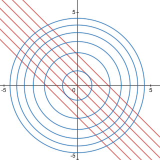
We can reason ourselves to the conclusion that the optimal solution lies at on the unit circle (which can be exhaustively verified, if not proven by plotting any other pair of coordinates within the constraint to see that they produce lower results). Furthermore, the minimum lies at the negative conjugate .
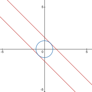
We can observe that, for any extrema along the constraint, our objective function will be tangent to the constraint. With this useful piece of information, we can restate our initial question to be the following: Find all locations where the gradient of the objective function and constraint are proportional; this will be our solution.
We can form a system of equations to solve this problem, starting with:
where is our constraining function, and is some proportionality coefficient called the Lagrange multiplier.
Expanding this equation and substituting the example definitions in our problem, we get:
To solve, we need the third equation: , given in the problem statement, which yields the familiar points:
and plugging them into our objective function confirms that the former point is the maximum that we're looking for.
This method enabled us to solve constrained optimization problems easily, but it's cumbersome to make a computer replicate this process. To streamline the approach, we'll take our system of equations unify all the necessary information into a single expression – The Lagrangian:
where is the right hand side of the constraint, in our case . To replicate the method of Lagrange multipliers shown above, we simply set the gradient of the Lagrangian to 0, and solve for its constituent variables:
which matches the same set of equations manually constructed with Lagrange multipliers. Therefore, it can be applied to any problem of the form
Example
Putting this all together, two-player Zero-sum Games have Nash Equilibria which can be expressed as a linear program, meaning the solution can be found in polynomial time. Given a game
where is the expected utility for player in equilibrium (the value of the game ), we expect by definition of a zero sum game that .
The construction of our linear program is then given by:
Note that all the utility terms are constant in the Linear Program while the mixed strategy terms and are variables.
Constraint (1) says means that for every pure strategy of , his expected utility for and given is at most : the optimal strategy.
For , those will be in 's best response set.
is subject to the same constraint, and the Linear Program will select in order to minimize . selects the mixed strategy that minimizes the utility can gain by playing his best response.
Constraint (2) ensures that is a well defined (or able-to-be-interpreted) non-negative probability (though reframing a problem with negative values into a probability is trivial via normalization). As mentioned early, the dual of this program can just as easily yield 's mixed strategy by flipping all mentions of with and attempting to maximize
To reach equilibrium rather than optimization, we introduce slack variables: for all and replacing the inequality constraints with equalities:
This is a general equivalent form of the first Linear Program since (5) requires only that each slack variable is positive, and the requirement of equality in (3) is equivalent to the inequality constraint in (1).
PPAD
Two-player General-sum Games are notably more challenging since the problem can longer be expressed as an optimization problem between tow diametrically opposed players. Furthermore, no know reduction exists from this problem to an NP-Complete decision problem.
Computing a sample Nash Equilibria relies on a different complexity class which describes the problem of finding a solution which always exists. This complexity class is known as Polynomial Parity Argument, Directed (PPAD).
Define: A family of directed graphs with each member of this family being a graph defined on a set of nodes. Though each contains a number of nodes that is exponential in , we want to boil this down to graphs that can be described in polynomial space. To do this, we encode the set of edges in a given graph as follows (with no need to encode the nodes, since they hold no value):
- Let and
be two functions that can be encoded as arithmetic circuits with sizes polynomial in . For every such pair of functions, let there be one graph provided that satisfies the restriction that there must be one node: zero parents. Given such a graph , an edge exists from node iff: and . We then have an exhaustive list of cases:
- zero parents, or one parent
- zero children, or one child
Per theorems of in- and out-degrees of the nodes in , we know that each node is either part of a cycle, or part of a path from a parent less source to a childless sink .
Returning to PPAD, this is a class of problems which can be reduced to finding either a sink or a source other than for a given .
As claimed earlier, such a solution always exists.
Proof: Because is a source, there must be some sink which is either a descendant of or is itself.
Theorem: The problem of finding a sample Nash Equilibria of a general-sum finite game with two or more players is PPAD-Complete.
Similar to proving NP-Completeness, the proof for this theorem can be achieved by showing that the problem is in PPAD and that any other problem in PPPAD is isomorphically reducible to it in polynomial time.
Further Reading
Gaus, Gerald F. "On Philosophy, Politics, and Economics," University of Arizona, 2008.
Moehler, Michael. "Why Hobbes' State of Nature is Best Modeled by an Assurance Game," Utilitas Vol. 21 No. 3, pp. 297-326, 2009, https://philpapers.org/rec/MOEWHS
Shoham, Yoav and Kevin Leyton-Brown. "Multiagent Systems: Algorithmic, Game-Theoretic, and Logical Foundations. Link
Karlin, Anna R. and Yuval Peres. "Game Theory, Alive." 2015.
Coding the Simplex Algorithm from scratch using Python and Numpy