ML 5: If My Mother Had Wheels She Would Have Been a Markov Chain Language Model

This post is under construction still. I can focus on precisely one thing at once for about 35 seconds before I become enthralled by the next thing. I feel like I've referenced the Joker a few too many times on here already, but "I'm like a dog chasing cars..."

Preface

Markov Chain Language Models – MLM, if you will.

The end goal of this article is to describe the process of building a predictive language model from scratch with Markov Chains. I hope to also mix in some style transfer elements so that we can train on grifty LinkedIn posts, and predict with Lovecraftian elements.

If my mother had wheels she would have been a bicycle.

Like all my poasts, this is mostly meant to be educational, and for my own edification –in this case, so that I never have to search back through my linear notes again– and hopefully it's understood that the final product is going to be kind of crummy, slow, and unimpressive relative to the technology available today. We don't care particularly about performance, accuracy, etc., since contemporary models and techniques significantly outperform Markov Chains. Nonetheless, I hope that anyone else reading is able to get something out of it!

Linear 👏 Algebra 👏 Review 👏

As mentioned above, accurate, performative text prediction is pretty close to a solved problem (at least for this task) (see RNNs, LSTMs, and, more recently, Transformer models), but we're just going to ignore all those advances in the field of NLP and pretty much count on our fingers in order to generate some moderately coherent text.

By count on our fingers, I of course mean that we'll be using Linear Algebra and –if you're incapable of simple arithmetic like I am– like two and a half legal pads of scratch work to verify that the examples included are in fact correct.

From a high-level perspective, we want to use a Markov Chain to determine how frequently some words in a corpus of text succeed another. Then, we can choose a seed word (or perhaps a phrase if we get that spicy), plug it into our model, and have it spit a sequence of words which tend to follow that word/phrase based on whatever training text we give as our initial "population."

If we trained it on my diary, a likely sequence stemming from the seed word "Cinnamon" might be

"Cinnamon Toast Crunch is obviously the best of the cereals. I don't know why anyone would ever contend that Cheerios..."

So, let's get into the math that we need in order to make this happen

Markov Chains

• A Probability Vector $p$ is a vector whose components are strictly positive, and whose sum over its components is equal to one:

• A Stochastic Matrix (or probability/transition matrix) $P$ is a matrix with all real entries, and whose columns are probability vectors:

An entry $m_{ij} \in P$ represents the probability of transitioning from the $j$th state to the $i$th state. Since it's an element of a probability vector, and thus a probability itself, the total probability of going from $j$ to any other state (including itself) must be 1.

• A Markov Chain is a sequence of probability vectors $\mathbf{x}_i$ together with a stochastic matrix $P$, where $\mathbf{x}_0$ is the initial state, and the subsequent state vector (the state vector at time step $i+1$) is given by:

Additionally,

A vector of a markov chain is called a state vector. The index $i$ of a state vector $\mathbf{x}_i$ represents the time step, so that vector describes the state of a system at time step $i$. Note that the above formula only holds for fixed transitions probabilities (it's not too difficult to model dynamic transition dynamics, by again leveraging some time step index $i$ for $P$, but we don't need to do that yet).

• A Steady State for a $n \times n$ stochastic matrix $P$ is a vector $\mathbf{q} \in \R^n$ such that

that is, the state vector does not change after being multiplied with the transition matrix.

Note that $\mathbf{q}$ is an eigenvector of $P$ for eigenvalue $1$, thus every stochastic matrix has a steady state vector!

To find the state state vector $\mathbf{q}$ of a matrix $P$, we perform the following calculation:

Matrix Multiplication Because, I Forgor

If $A$ is an $m \times n$ matrix, and $B$ is an $n \times p$ matrix:

then $C = AB$ is an $m \times p$ matrix s.t.

• The $c_{ij}$ entry of the product is given by the term-by-term entries of the $i$-th row of $A$, and the $j$-th column of $B$, that is: the dot product of those row/column entries.

• The product is defined iff the dimensions align:

• If $A, B$ have dimensions $m \times n, p \times q$, then $AB$ is defined if $n=p$ and $BA$ is defined if $m = q$. Otherwise, the product is not commutative

Example

Suppose 3% of the total population of a system lives in $A$ and the rate of migration to and from $A$ is constant according to the following stochastic matrix:

From here, we send(?) $P - I$ to Reduced Row Echelon form. I've included annotations for the arithmetically incompetent (recall that this is myself). I always got annoyed when my linear professor would also bungle this step; just goes to show: who among us is an abacus. I know some of you psychos can like stare at html and just see web page, but I forgot my times tables a long time ago, so bear with me:

Our steady state vector $\mathbf{q}$ is any solution which, when multiplied with our resultant reduced matrix, will be the zero vector of corresponding dimensions:

One such solution is:

for which we factor out the second component to make the vector flexible and identitive. We also rationalize its entries such that its sum is equal to 1 to maintain the handy-dandy probabilistic properties.

• A Regular stochastic matrix is a matrix $P$ for which there exists some power $k$ such that $P^k$ contains no zero entries. If $P$ is a $n \times n$ regular stochastic matrix, then $P$ has a unique steady state vector $\mathbf{q}$. If $\mathbf{x}_0$ is any initial state vector, then the Markov chain $\mathbf{x}_k$ converges to $\mathbf{q}$ as $k \rarr \infty$.

Example

Consider the following example of how we can compose this vocabulary and what kinds of questions we can answer with them.

Given a system composed of nodes $A, B, C$ with the corresponding transition probabilities $P$, and the initial state vector $\mathbf{x}_0$:

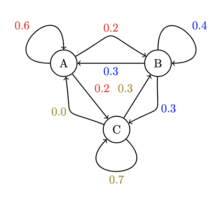
We can interpret $P$ according to this diagram as follows, with the columns corresponding to the source/from, and the rows corresponding to the target/to – that is, there is a 0% chance that $C$ ever goes (directly) to $A$:

And we can ask and answer some questions like "What is the state vector at time step 1?":

What does this have to do with text prediction???

Rather than considering states, populations, and transition dynamics we can instead use these same properties of markov chains to consider words and the frequency with which they appear in sequences with one another.

Code

Base Model

What's your favorite data structure and why is it a Bag? Sorry to disappoint, but that old school openDSA example is pretty much what backs our markov chain. We can and will spice it up a bit for the sake of observability within the model, but the base model for text generation (prediction might be a bit generous for how rudimentary this ish is about to be) is pretty much a sack of technicolor marbles with a sparse amount of pointers from marble to marble. In fact, the base model can be implemented in like 8 lines using python's Counter collection, but again, we're going to step back and do this a bit more artisanally for the sake of understanding and so that when we do decide to graduate from Bags to something a bit fancier, we have more control over how things work.

The approach I'm going to opt to use for the base model is as follows:

1. ingest a ton of "training data"
2. generate a ton-minus-one bigrams of all the adjacent word sequences in the data
   • eventually, these could be generalized to be n-grams, a larger window of context, so to speak, but I'm gonna keep it simple for now
3. keep track of how often each word follows another word
4. select a starting word and sample from its successor words
5. repeat until we've generated a satisfactorily long sequence

Discrete Probability Distribution

Now, we could just throw every $i+1$th word into a list associated with the $i$th word, producing something like this

markov_chain = {
    word1 -> [word2, word3, ..., word2 again, etc.],
    word2 -> [...],
}

but then we'd have to tack on some overhead junk later on if we ever wanted to introspect into our "tree" of possible sequences to see the frequency with which each word appears (I say overhead, but it'd probably be as simple as markov_chain[word1].count(word2), but maybe we'll want something juicier down the line?).

So, instead of just using dictionaries and lists, we're going to represent our markov_chain as a dictionary of DiscreteDistributions which is just going to be a dictionary with some additional functionality to easily sample from.

This is hardly an original implementation of this idea, I yoinkied this from a course assignment, and I'm pretty sure it's part of the boiler plate code for a bunch of Berkeley assignments, but it's so ubiquitous that a reference seems unnecessary

# DiscreteDistribution
import random
import numpy as np

class DiscreteDistribution(dict):
    """
    A DiscreteDistribution models belief distributions and weight distributions
    over a finite set of discrete keys.
    """
    def __getitem__(self, key):
        self.setdefault(key, 0)
        return dict.__getitem__(self, key)

    def copy(self):
        """
        Return a copy of the distribution.
        """
        return DiscreteDistribution(dict.copy(self))

    def argMax(self):
        """
        Return the key with the highest value.
        """
        if len(self.keys()) == 0:
            return None
        all = list(self.items())
        values = [x[1] for x in all]
        maxIndex = values.index(max(values))
        return all[maxIndex][0]

    def total(self):
        """
        Return the sum of values for all keys.
        """
        return float(sum(self.values()))

    def normalize(self):
         # can't divide by 0
        total = self.total()

        # only normalize if the total isn't 0
        if not total == float(0):
            for k in self:
                self[k] = float(self[k])/total

    def sample(self):
        weights = [ float(w)/self.total() for w in self.values() ]
        rand = random.random()

        for weight, key in zip(weights, self.keys()):
            if rand <= weight:
                return key
            else:
                rand -= weight

For the base model, we only really need the sample method, but again I'd like to think that this is a symptom of foresight.

Everyday, I await the opportunity to say "oh geez, I wish I had an argmax right about now."

From here, we can follow the rough outline provided above, starting first with the ingestion of data. Future peter will scrape a bunch of gross LinkedIn humble-flexxing posts, but for now, I'm going to use a bunch of Shakespearian sonnets.

I took the liberty of manually cleaning my copy of this file so it doesn't have the licensing meta information in it. Not because I think piracy or stealing is cool (it is), but because, in the off chance that our randomly selected seed phrase is "ELECTRONIC," I don't want produce the Project Gutenberg license disclosure. That shit isn't even in Iambic Pentameter.

def load_corpus(fname="data/sonnets.txt"):
    """load a file and convert it to a list of words"""
    corpus = open(fname, encoding='utf8').read().split()
    return corpus

Next, we generate our bigrams:

def get_bigrams(corpus):
    len_corpus = len(corpus)
    for i in range(len_corpus-1):
        if i % (len_corpus/5) == 0:
            print(f"{i}/{len_corpus}")
        yield(corpus[i], corpus[i+1])

Now, we create our markov chain and populate it with Discrete Probability Distributions over all word sequences of length two:

corpus = load_corpus()

markov_chain = {}
bigrams = get_bigrams(corpus)

for w1, w2 in bigrams:
    # if we've seen w1 before
    if w1 in markov_chain:
        # if we've seen w2 after w1
        if w2 in successors[w1]:
            # increment the count of w2 after w1
            successors[w1][w2] += 1
        else:
            # else we haven't seen w2 after w1
            successors[w1][w2] = 1
    # else we haven't seen w1 before, so make a new entry for it
    else:
        successors[w1] = DiscreteDistribution()
        successors[w1][w2] = 1

seed_word = np.random.choice(corpus)

# naive filtering to try to get a capital word
while seed_word[0].islower():
    seed_word = np.random.choice(corpus)

chain = [seed_word]
n_words = 50
for _ in range(n_words):
    current_word = chain[-1]
    chain.append(successors[current_word].sample())

print(' '.join(chain))

print(f"seed_word: {seed_word}, successors: {successors[seed_word]}")
n_successors = len(successors[seed_word].keys())
print(f"n_successors: {n_successors}")

Running our lil script I get the following output. (I held the hand of the base model by reformatting this to better resemble a dialogue):

---
Montague that you hope to the Queen's dram of Bohemia?

MARINER.
    I would have a field We will score When most magnanimous as a
    man. Tyb. Mercutio, let's make his gorget, Shake in mind Still
    thus, Yet he will thank it, and He is meet thee, strumpet!

DESDEMONA. You might too
---

seed_word: Montague
successors: {'shall': 1,
             'that': 1,
             'as': 1,
             'hath': 1,
             'our': 1,
             'moves': 1,
             'is': 2,
             'and': 1,
             'That': 1,
             '[and': 1
            }
n_successors: 10
KEY     SAMPLED OCCURRENCE
--------------------------
shall   0.107
that    0.101
as      0.084
hath    0.09
our     0.082
moves   0.098
is      0.162
and     0.086
That    0.091
[and    0.099

For the seed word Montague, we can see that there aren't a ton of common successors. In fact, the most common of the 10 –is- is only doubly as likely as any of the other candidates. But, thanks to the DiscreteDistribution wrapper class, we can see that this appropriately reflected in the sampling frequency, with is having roughly twice as high of a sampled frequency of 1.62 than the other successors which each have about 1/11th of a chance to be selected.

Observation

So, a couple of obvious comments.

• Low hanging fruit item 1: We'll get more variety in our output the larger of a "training" data set we choose. More word succession combinations, more data, more gooder. QED.
• Obvious caveat to low hanging fruit: The smallest amount of effort put towards preprocessing this data would greatly improve the coherence or semblance of grammar, even more so than just having a yuge corpus. One drawback of using poetry or a screenplay is the somewhat arbitrary capitalization of letters and even entire words (an extension of the need to remove the license which was initially duplicated 218 throughout this file). If we took the time to filter and clean this data such that only proper nouns and the starts of sentences were capitalized, we might converge towards something that doesn't sound like drunken screed, but hey– I chose Shakespeare for a reason!
  • While, for the sake of generalizing this model, it probably makes sense to also trim punctuation so that words like [and and and are considered the same will also increase the variety of our model, the existence of this punctuation is actually doing a lot of favors for us right now by constraining our output to be somewhat structured, with vague sentence forms.
  • If you run the model enough, or even just boost the output sequence length, you might encounter scene transitions, or the termination of one sonnet and the start of another! While this is pretty good, we might do better by encoding special tokens to replace this punctuation which yields structure such that words can be words, and syntax can be syntax. But if my mother had wheels...
  • I took the time to do some preprocessing along these lines for the input to 16 | ML 3.5: A Post by Peter?, but notably didn't take the time to replace that somewhat-necessary syntax with embedded tokens to indicate terminal points, or complex grammar of any kind, which is why it palavers. This is evidenced by the open parentheses, quotations, and lackadaisical use of commas and periods. It's well-nigh a miracle that the RNN used for that text generation managed to close the one LaTeX sequence at all, but honestly I chalk that up to severe overfitting rather than any notion of learnedness, which is a legitimate issue with small datasets.

Review / match up with the Linear

So, where to from here? With this very crude base model, we can now tackle some more exciting challenges.

Style Transfer

Resources

• https://www.kdnuggets.com/2019/11/markov-chains-train-text-generation.html

• https://ericmjl.github.io/essays-on-data-science/machine-learning/markov-models/