Abdicating to the Algorithms: Solving the Redistricting Problem

1. Introduction

In light of the technological advances made in the past five and a half decades, is there any remaining reason why voters, taxpayers, and legislators should settle for the flawed, politically corrupt, or otherwise excessively litigious processes by which most states currently determine their district boundaries? The empirical data gathered by researchers on the performance of computational models would suggest not. In order to understand the current issues surrounding gerrymandering, it is first necessary to understand the task of redistricting, how it varies from state-to-state, and how the Supreme Court's involvement over the years has only muddied the waters for district drawers. With the requisite background knowledge of precedent, custom, and Constitutional constraints which inform contemporary institutions tasked with proposing new district maps, an examination of more recent reapportionment disputes will help contextualize a discussion of computational models. Following a historical overview of the literature surrounding State of the Art models from the 1960s to the present, I introduce an argument for why they should be adopted in favor of the inferior institutional means of redistricting as well as discussion of the ethical implications that need to be considered when suggesting an abdication of control at this scale. In this paper, I argue that the problem of redistricting is better solved by computational models than by humans, and that their adoption is not only an ethical and logistical possibility, but rather a vast improvement over current techniques.

2. Summary of Redistricting Processes

Before describing the many issues surrounding gerrymandering and reapportionment, it is first necessary to establish a common baseline of knowledge about the redistricting process. Every ten years, following collection of the national census data, states are tasked with redrawing their congressional and state-legislative districts to better reflect the updated population distributions. Article 1, Section 4 of the United States Constitution charges these state legislatures with the responsibility of determining the “Times, Places, and Manner of holding Elections for Senators and Representatives,”¹ but does not specify how they are to carry out the task. As such, particular mechanisms and processes used by the state governments vary. In many states, the legislatures draw both the congressional and their own legislative districts. In eight states, advisory bodies composed of state legislators or elected officials are responsible for proposing at least one of the two maps to the state legislatures for approval. Four states utilize independent commissions –a group excluding public officials and current lawmakers– selected by some independent entity to draw both maps. In any case, the states' Governors typically reserve the right to veto a plan passed by the legislature with the exceptions (for congressional maps, legislative maps, or both) of Florida, Maryland, Mississippi, Connecticut, and North Carolina.² While many of the maps that these various institutions draft may pull from insights provided by a computer program, currently no state governments formally rely on computational means of redistricting. As a result of the largely human-based processes described above, it should come as no surprise that legislators' personal interests, namely to pursue a successful reelection, often conflict with the motivations of an otherwise neutral actor issued the identical task of reapportionment. Enter the gerrymander.

3. A History of Gerrymandering and the Law

While gerrymandering has been further proliferated by varying degrees of judicial efforts to resolve political disputes which have arisen from district boundary proposals, its application within the United States predates the inception of the nation itself. Discriminatory reapportionment practices are documented as early as 1705, since the adoption of popular election by districts in America, and continuing through the remainder of the colonial era up to the present day.³ The term originates from a political cartoon which appeared in the Boston Gazette in March of 1812, criticizing Massachusetts governor, Elbridge Gerry, for approving a district proposal whose district of South Essex was intentionally and peculiarly shaped (resembling a salamander) to benefit the Democratic-Republican party.⁴ Hence, the gerry-mander. Whereas some critics argue that the wrongness of the gerrymander supersedes political motivations and is rather the violation of the integrity of geographical unity, or a peculiar arrangement formed intentionally for partisan advantage,⁵ for the purpose of this paper I will subscribe to the definition presented by Stuart Nagel in his seminal paper, Simplified Bipartisan Computer Redistricting, which demonstrated the viability of computer programs to solve the issue of redistricting. He defines gerrymandering to be “the deliberate drawing of district lines so that one party wins a percentage of districts that is substantially greater than its percentage of voters.”⁶

In his widely cited 1907 dissertation, The Rise and Development of the Gerrymander, Dr. Elmer Griffith catalogues a litany of examples of partisan gerrymandering throughout the 18th and 19th Centuries. Interestingly enough, he asserts that perhaps the most successful of these early gerrymanders preceded that which led to the caustic nickname used against the Democratic-Republicans of 1812. He describes a gerrymander occurring fourteen years prior, where Federalists in New Jersey arranged the legislative districts such that they carried four of the six districts in an election which would have otherwise certainly gone in favor of the aforementioned Democratic-Republicans if the vote were carried out at large.⁷ This example is mentioned to underscore the fact that the gerrymander, while partisan in intent, is party-agnostic in application. Griffith's dissertation details over thirty such examples executed at the hands of each political party which rose and fell during the time frame he covers, bringing the “evil” practice into the fold of established fair play between agents and institutions vulnerable to the machinations of human nature.

As a result of the numerous efforts, successful or otherwise, to use the gerrymander, several states amended their constitutions with prohibitive language and requirements including provisions for: contiguity, compactness, county indivisibility, limiting reapportionment to be a once per ten years affair, and –in some cases– dismissing the use of districts altogether. Throughout the late 19th and early 20th Century, many states enacted “silent” gerrymanders by refusing to partake in reapportionment to reflect new census data.⁸ Similarly, gerrymandering tactics of composition, formation, and law were commonplace for several decades. Tactics such as proposing boundaries which would thinly spread a political opponent's voter base across several districts, or alternatively, forfeiting a single district by drawing lines so as to concentrate as many of their prospective voters as possible into a single district, or stretching districts into “unnatural” shapes to include a specific voter base, or amending the state's constitution to limit the amount of counties that could be present in a district –effectively making reapportionment impossible– were all implemented across the nation. As Dr. Leroy Hardy notes, many of these Constitutional gerrymanders were the result of the dated constitutions which predated the major rural-urban conflicts which began unfolding following the turn of the Century. These practices did not go unnoticed, and eventually the Supreme Court intervened to rule on the Constitutionality of such practices.

It was not until later in the 1960s under Earl Warren's tenure as Chief Justice, though, that the Supreme Court started to play a more active role in enforcing regulations to combat the numerous forms of gerrymandering manifesting in these urban-rural hotbeds of conflict. Several landmark cases forced regulations to become more standardized, albeit still tenuous. For example, the cause of one of the first modern Supreme Court rulings on the issue in Baker v. Carr (1962) resulted from a silent gerrymander which took place in Tennessee. The Shelby County district had not been reapportioned for sixty-one years and had quadrupled in size (153,557 in 1901, to 627,019 in 1962), whereas another county district remained stagnant with a population of just under 15,000 throughout the six decades in question. As a result, the federal courts intervened to strike down the state's constitutional stipulations which had allowed the silent gerrymanders to take place, marking the beginning of the Court's willingness to deem issues of legislative apportionment judiciable. In the ruling of Reynolds v. Sims in 1964, the Court found that the extreme disparities in some of Alabama's district's populations violated the Equal Protection Clause assuring all citizens substantially equal legislative representation. Thus, the Supreme Court enacted what has come to be known as the “one person, one vote” rule as well as the decennial status which mandated reapportionments to take place not more or less than once per ten years.^9,10 But, as we will see shortly, the precise standard by which the Equal Protection Clause was enforceable was severely absent from the Court's opinion.

These advances made by the judiciary still failed to establish common, objective rules for reapportionment, and legal disputes have continued through to the 21st Century as the Court's involvement and opinions became increasingly opaque but firm due to their reluctance to rely on a reasoning tied to partisan proportionality.¹¹ Nevertheless, the Supreme Court remained resilient in its compulsion to pass judgement on issues of apparent gerrymandering. In 1986, Alexander Bickel asserted that the stringency of enforcement of the criterion of population equality had, in fact, enabled state legislatures to participate in and justify gerrymandering districts to meet these requirements imposed by the Court.¹² Further complicating the matter, in the 1983 case of Karcher v. Dagget, the Supreme Court invalidated New Jersey's redistricting map on grounds of its deviation from the ideal average district population by 0.1384%. As Michell Browdy notes in her essay advocating for replacement of legislative processes entirely with computer models, this deviation is within the margin of expected statistical error for the census data from which the target average population was calculated. She adds that Justice Stevens' concurrence explains that the “awkward” ruling was determined because “the New Jersey plan appeared on its face to be gerrymandered.”¹³ Thus, the Court dismissed a redistricting plan for its appearance, whilst alluding to arbitrary figures.

Similarly, but with the opposite determination of a prima facie case of unconstitutional gerrymandering, in Davis v. Bandemer (1986), the Court's ruling arguably did more harm than good. The decision, which overturned the lower District Court's ruling, found that the discriminatory effect of Indiana's 1981 apportionment against Democratic legislators did not surmount the threshold required for an on-its-face violation of the Equal Protection Clause.¹⁴ However, elaboration of the objective standards of this threshold in the Court's opinion were not forthcoming. By repeatedly ruling on such cases without providing concrete standards for legislatures, commissions, or advisory bodies to leverage when tasked with drawing new district boundaries, the Supreme Court effectively transformed the reapportionment process into a minefield of conflict. Additionally, in each of these cases, the Court expanded the scope of its purview from a willingness to rule on the legality of states' Constitutional requirements for reapportionment to prevent silent gerrymanders (Baker v. Carr) to the conclusion that rulings on the political nature of an instance of gerrymandering were justiciable (Davis v. Bandemer). While this expansion was necessary in order to correct the unfair tactics being employed at the state level, the implications were nebulous and ultimately opened the door to additional vectors of legal dispute, and made the processes of redistricting increasingly litigious.

The issues with the current redistricting process(es) are twofold. First, the ambiguous legal constraints which have become embedded in the institutional mechanisms have made the process rife with conflict which, as observed above, necessarily requires judicial intervention. Furthermore, these issues have not been resolved in the 21st Century^15,16 and Justices of the Court itself have criticized the expansion of the Court's purview, with Justice Scalia writing in the plurality decision of the more recent case of Vieth v. Jubelirer (2003), that the Court should declare all claims related to political gerrymandering as nonjusticiable since no court had been able to find an appropriate remedy to political gerrymandering claims in the two decades since Davis v. Bandemer.¹⁷Second, the processes themselves, party- and legal-disputes notwithstanding, are severely imperfect as we will see when discussing even the earliest computer programs aimed at achieving improved results.

4. A Survey of Research into Computational Redistricting Models

Though the picture painted is bleak, opportunities for improvement are frustratingly achievable. In this section, I aim to present an overview of methodologies used by a selection of models which outperform human institutions when it comes to the task of reapportionment, highlighting the efforts of a few key researchers in the field whose work demonstrates that the problems of gerrymandering and efficient, acceptable redistricting are solved by computer programs, and has been since before the passage of the Voting Rights Act.¹⁸

The goal of this survey is to illustrate the general advantages of models along four axes of superiority: reviewability, transparency, speed, and correctness. By reviewability, I mean the deterministic nature of the models discussed; the same set of inputs should result in the same output of the program. Similarly, with respect to transparency, it is safe to assume that the underlying source code of the program or model would be visible to the public, and to the judiciary as needed to adjudicate disputes. This implies that the decisions which govern the program's output can be traced line-by-line through the code, translating the focus of the question of motivation from the process itself to the inputs. This is a key advantage raised both by Nagel¹⁹ and by Browdy:²⁰ that the models themselves are agnostic insofar as the criteria that they optimize for can be as non-partisan as possible, instead being guided by legal standards (one man, one vote rule) and customs (contiguity and compactness for fear of prima facie gerrymandering). Speed describes the time and cost necessary to generate a solution, and correctness is defined relative to the criteria which each model optimizes for compared to the score an institutional map would receive when subjected to the same calculations. Measures of correctness typically rely on some combination of deviation from average district population, compactness, respect for geographical features of import, and maintenance of political balance. With these criteria in mind, a discussion of a selection of models demonstrates that computational methodologies consistently outperform institutional efforts to solve the problem of redistricting.

Following the popular reception of his paper Simplified Bipartisan Computer Redistricting, Professor of political science Stuart Nagel published an addendum surveying what was considered to be the state of the art in computational efforts for aiding the redistricting process circa 1972.²¹ His three eponymous criteria include 1) cost and time effectiveness,²² 2) adherence to the Court's one-person-one-vote rule via enforcement of district population conformity as well as rules for compactness and contiguity, and lastly, 3) that the resulting reapportionments should minimize the unhappiness of incumbents, maintaining party balance and the status quo in order to be acceptable to the impacted legislators.²³ While the criteria he used in developing the first model discussed in his 1965 paper laid the groundwork for several subsequent models, they were by no means the de facto standard for success at the time²⁴ His survey describes a variety of approaches to the problem, some of which satisfy his normative criteria more than others.

He mentions the mathematical success of some approaches which utilized either geometric divisions^25,26,27 or solutions which utilized a transportation algorithm known to be capable of solving linear systems of equations by which the input to a redistricting problem can be represented,²⁸ but notes that “While the latter approaches are aesthetically satisfying, the simplifying assumptions [respecting the status quo and geographical/county lines] are violated in practice.”²⁹ Thus, he concludes that the approach described in his paper –“moving-and-trading”– is normatively superior with respect to his criteria as it was designed with those principles in mind, and therefore more closely resembles the human approach, offering better and more intuitive solutions. In the example problems he describes, both the trivial 3-district problem and the larger 1963 Illinois problem, the program resulted in districts which saw a decrease in deviation from the ideal average population at the expense of minor compactness penalties.

The aforementioned “moving-and-trading” algorithm presented in his 1965 paper is both surprisingly intuitive, performative, and obtuse, serving as a testament to the feasibility of the adoption of a more sophisticated contemporary model for use. Simplified Bipartisan Redistricting describes this “moving-and-trading” program, written by the geographer Waldo Tobler, which computes accurate reapportionment patterns in a matter of seconds, reflecting the values determined users. These values are provided via at least three punch cards. The information on the first “parameter” card indicates baseline information for the program,³⁰ as well as the values (reapportionment preferences) of the user.³¹ Each subsequent punch card input would contain the data for each indivisible unit describing their populations, geographical coordinates (for computing compactness), current district membership, a list of geographic neighbors (used for computing contiguity), and the number of votes for each major party in that district.

What follows next are what Nagel candidly titles the “Starting, Moving, Revising, Proportionality, Residual Contiguity, and Output Parts.” The primary mechanism of the program is to minimize the badcount –the number of districts which exceed the MAXCUT parameter which the user provides as one of his preferential values– and the compactness penalty of each district weighted by the W parameter. This is achieved within the “Moving” and “Revising Parts,” by attempting to move each unit within a district to every other district either sequentially or simultaneously. Such a move can only be made if moving the unit does not break the contiguity of either the host or destination district; and the host district retains at least one other indivisible unit after the move, lest the district be destroyed. A move is only kept if, following a subsequent computation of the badcount and compactness, the move resulted in an improvement. In this way, the initial steps towards minimization of this heuristic penalty are minimized. If the number of moves made was non-zero, the algorithm repeats this greedy³² $O(n^2)$ calculation³³ until no more moves which result in an improvement in terms of the heuristic can be made. The Proportionality Part involves determining the preponderance of the vote that each major party would receive based on the baseline number of votes to each party indicated by the parameter cards.34 The Residual Contiguity Part simply verifies that the consummate trades between districts did not invalidate the contiguity of any of the constituent districts, and lastly the Output Part simply details the movements and trades made, as well as the final heuristic penalty values relative to the initial characteristics computed in the Starting Part. The findings of Nagel's iconoclastic paper show that this technique can be used to compute numerous solutions to the redistricting problem which are superior to those generated by the competing human institutions.

As alluded to earlier, the promise of this particular program can be partially attributed to its inefficiency relative to standards of modern computing. Nagel notes that each run of the program costs approximately $5.63 and takes 81 seconds to complete.³⁴ Additionally, he references dangerous and inefficient programming techniques –namely the use of the go to instruction– which would be famously criticized by A.M. Turing award winner Edgar Dijkstra just four years later.³⁵ Refactoring the program presented in Nagel's paper, written in one of the first programming languages, Fortran, with modern computing practices and hardware in mind could drive computational costs and execution time to zero, utterly dispensing with the time and cost concerns Nagel presents as an initial constraining criteria in his 1972 publication. Needless to say, the developments in computing over the nearly-six-decades that have elapsed since the release of the program which Nagel describes eliminate the concerns presented about availability of computational resources.

Next, I present an expedited review of the methodology and results of a selection of newer models which both expand upon and deviate from Nagel's criteria and Tobler's technique, optimizing for geographical features, and margin of victory in districts to achieve their measures of fairness. Advances in both computational hardware and theory have enabled the development of increasingly complex and efficient models.

First, a study conducted by Richard Morill in 1976, in which “The hypothesis that computer models would be inferior to human judgement was rejected.”³⁶ Morrill compares the actual outcome of Washington state's congressional redistricting efforts in 1972 against those computed by a model which optimized for both district population equality and district compactness as defined by travel distance from boundary to center. An important critique which he raises is that Tobler's move-and-trade program is not practical for initial configurations which have undergone significant population change.³⁷ Crucially, therefore, the model he describes does not initialize the new districts to resemble the old districts (in an effort to maintain the status quo), instead simply selecting district centers (either randomly, or intelligently according to existing district or county centers), and finding a set of equally populous districts such that the aggregate travel to their respective centers is the minimum possible, while also satisfying legal constraints of population equality and compactness. Despite this forfeiture of Nagel's criteria for maintaining the status quo, Morill notes that “The integrity of cities and counties is automatically favored because they constitute so many of the origin areas.”³⁸ The objective function which his model employs measures distance according to a transportation network of nodes which better reflects infrastructural travel, as opposed to a straight line, as-the-crow-flies distance, which can be weighted according to geographical features of interest, such as minority populations or political unity. In this way, he is able to compare the district maps along the axes of efficiency (compactness and distance minimization) as well as reasonableness (the extent to which the plan respects geographical regions).

He then compares three computed maps, optimized for airline distance, road distance, and time distance (where paths and subsequent district lines were modified to preserve the integrity of specified geographical features). In cases where the computed distances were not the minimum, district origins were manually re-centered, and then passed as input for a second iteration of the program. For each improved map, Morill found that the district centers and shapes were highly similar to those which were actually adopted in 1972 but qualifies this finding with the following insight:

The fact that in many respects the plans are not markedly different should not be attributed to the hypothesis that man is as good as the machine, or vice versa, but that the peculiarities of population concentration in Washington tend to restrict the number of reasonable alternatives.³⁹

Additionally, he concludes that the computed maps were preferable to the actual map in terms of efficiency and reasonableness. Just over a decade after the initial exploration into computer-aided reapportionment, Morill's findings underscored the feasibility of the application of these improved models, going as far as to suggest that they might have been consulted in Washington if not for the severe time constraints imposed by the 1972 and 1974 elections.

Lastly, an examination of a contemporary study published by two students from Cornell University earlier this year, titled Fairmandering: A column generation heuristic for fairness-optimized political districting. Whereas the previous two programs or models optimized for efficiency, reasonableness, legal constraints, and/or maintenance of the status quo, the model presented by the Gurnee and Shmoys optimizes for a fairness heuristic called “efficiency gap” which is a measurement of the margin of victory for any given district: “A fair district plan ... is one that, on average, calibrates electoral outcomes with the partisan affiliation of a state to minimize the number of wasted⁴⁰ votes.” Given the amount of data available to researchers and institutions, the authors assert that the scope of the current problem is vastly larger than the earlier two examples, and that “exact optimizations methods are intractable for large problems.”⁴¹

Instead of an exact, iterative approach, they describe a more sophisticated approach which, given a set of geographic polygons and their respective populations, generates partitions of those polygons (analogous to Nagel and Tobler's units), such that each district is population balanced, geographically contiguous, and compact. Their model applies a set partitioning algorithm called “column generation”⁴² to the huge set of geographical polygons in order to generate an ensemble of over 1 Trillion possible district configurations by recursively splitting the total region into subregions, and partitioning those a number of times as well. This generates a tree of several possible configurations where the children configurations of the tree are governed by the structure of the higher nodes (which represent the earlier partitions made to the initial region).

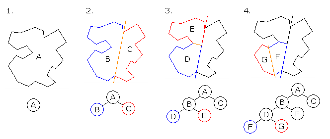
(Figure 1 - Example of a Binary Space Partitioning tree similar to what is created in Fairmandering)

Noting that the overwhelming majority of the distribution of possible configurations which are arbitrarily generated by the recursive partitioning process are likely unsuitable,⁴³they sample from the tail-ends of the distribution to populate what they refer to as a “Stochastic Hierarchical Partitioning Sample Tree.”⁴⁴ The result is a curated subset of possible solutions from which they can once again sample and score with their objective function in order to quantify desirable characteristics while ignoring. Using a method called integer programming which Nagel alluded to in his 1965 paper,⁴⁵ each partition is scored according to the split size, capacity, and position. The fairness of a possible district (which is represented as a column within the tree), is computed according to the aforementioned efficiency gap criteria. The “Master Selection Problem” involves selecting columns from the curated tree which meet some predefined threshold for admissibility.⁴⁶ Furthermore, despite the absence of explicit instructions in the algorithm's objective function to highly score districts which respect geographical features or political influences like Tobler or Morill's models, the authors note that:

In a state where a fair solution exists, there are typically a large number of alternative fair solutions. Since there are many other desirable properties of district plans to trade off, one can filter the range of candidate plans to those that meet a requisite level of fairness, and then consider other properties such as competitiveness, maintaining political boundaries, or not separating communities of interest.⁴⁷

In addition to finding that such a method computes several optimal reapportionment solutions, Gurnee and Shmoys show that compactness and fairness⁴⁸ are orthogonal characteristics of district map, thus quantifying the challenge illustrated in Section 3 with respect to the Court's ambiguous and awkward standards. While the complexity of their approach poses numerous ethical questions, the sophistication and success of this model serves as a benchmark for the possibilities of modern computer-aided redistricting.

5. Ethical Considerations

This section aims to address points of contention surrounding the use of- and advocacy for- computational models for the problem of redistricting. Questions of implicit and explicit bias, verifiability, and obfuscation are all called into question by the proponents of these models. Additionally, I offer arguments in favor of their widespread adoption in terms of the prior criteria used to evaluate models.

First, to acknowledge points of contention. It is understandable and encouraged that cautious readers and members of the public be hesitant to cede the responsibility of redistricting from their democratically elected representatives to computer programs. Without sufficient background education or training, how are they to trust the inner workings of a computer program with their interests as voters or as constituents whose welfare is ward to their representative? If their representatives are able to come to consensus on suitable criteria, values, or definitions of correctness, as well as guidelines for those meta-values pertaining to population equality, geographical compactness, and party influence dictating the implementation of a program, then transitively, by the nature of the republican democracy that they participate in, voters should accept the adoption of models for these determinations. The many empirical studies researching this question already demonstrate that these programs can be trustworthy and superior.

Additionally, it is possible to separate individuals' motivations from the implementation of the program and also from outcomes by the use of models. Nagel argues that by explicitly embedding value claims in the model, the only avenue for additional bias is in the form and format of the input to the model itself.⁴⁹ By codifying those values in a model, they are instantly available to other parties for review and rejection if those values are unfit. As Morill candidly notes in the description of the model he reviewed when comparing Washington's 1972 outcomes, “A distance modifier might be employed with respect to race, reducing apparent distance within a community, and with respect to integrity of cities or counties, ... A risk of subjectivity and arbitrariness is introduced in this step.”⁵⁰ Once again, however, the distance modifier is baked-into the model, and the metric which is weighted (in this case: racial demographics) is a tunable externality of the model itself. It can be removed, or counterbalanced by another opposing interest to reach a new set of boundaries which is still enticing to the individuals who hold the power and still a net-improvement over prior, institutional configurations. Thus, institutional motives can only manifest in definitions of model criteria and, in some cases, the input to a model. However, it is unlikely that bipartisan legislatures would agree to a model which implements a value or bias in a way which disproportionately benefits one party at the expense of another, and likely illegal in cases where parties would adopt values for model implementation which exploit protected demographics. Furthermore, as observed in the model survey, seemingly any model implemented in good faith can produce multiple reapportionment solutions which are more correct and more fair for the voters. Provided that discussion of models is introduced in states with even semi-competitive representation, the only reason why they ought not be accepted is because of incumbent politicians' fear of losing their seats under what must be –by some definition– a fairer reapportionment.

Another pain point lies in the complexity of the proposed models. While “salt of the earth” algorithms underlying models such as the briefly noted pies-slices, diminishing halves, shortest-split-point, and other geometric or mathematically optimal techniques⁵¹ are arguably the most transparent and intuitive, they fail to satisfy the necessary criteria of being politically feasible. Therefore, some transparency, in terms of the comprehensibility of a model to the voting public, must be sacrificed in order to meet this pragmatic constraint, lest they fail to be logistically feasible. However, the severity of this concession is tempered by the criterion of reviewability. By enforcing a rule-based, deontological implementation of these models (especially deterministic models), the consequences of each model should be evident to the stakeholders, regardless of whether or not it is fully understood how a model arrived at a solution. As Browdy argues, “reviewability should make it possible to require redistricting to meet manageable, meaningful judicial standards,”⁵² whereby the threshold for satisfiable reviewability could be determined by the state legislatures or alternatively (perhaps inevitably) the higher Court. The argument in favor of using models is not that the value gain lies in the elimination of bias and motivation, but rather that they are made explicit in a definition of fairness, while also being public and reviewable in their implementation.

The latter two advantages gained from the adoption of these models directly correspond to the two remaining criteria used to compare models in the previous section: speed and correctness. As observed in the survey of only a handful of computational approaches published in the past fifty-six years, all computational models are more efficient, in terms of both time and monetary cost, than any sincere institutional approach. In describing his motivation, Nagel asserts that

Those responsible for redistricting should not become so bogged down with desk calculators and pencil-paper figuring that they run out of time or become paralyzed and have to hold an at-large election (as in Illinois), call for a national constitutional convention (as in California), or consume tens of thousands of dollars (as in New York) on a redistricting that a computer could have done for a few hundred dollars.⁵³

With labor and computational costs adjusted up and down respectively, this argument is ever stronger in the modern litigious and technological era. As Gurnee and Shmoys point out, “In 2021, 428 congressional, 1938 state senate, and 4826 state house districts will be redrawn, cementing the power balance in the United States for the next decade,”⁵⁴ and hundreds if not thousands of alternative reapportionments which currently are, or will be, superior to those produced by institutions can be computed in a negligible time frame. Furthermore, with respect to correctness of computed maps, justifications for any institutional proposal which deviates from the correctness of such a map by any metric other than disruption of the status quo are moot. Even if those biases and motivations are embedded into the value parameters of a model, the resultant reapportionment is still more equitable and fair for both the minority and majority parties. Only the most base and selfish motivations of elected officials seem like rational counterarguments when combinations of every other reasonable metric –equality, compactness, margin of victory, etc.– can be improved upon by a computer program.

6. Conclusion

As illustrated in the historical summary of legislatures' various failures to fairly carry out the task of redistricting, as well as how the Court's involvement in the past two Centuries has only further complicated the matter, the current processes of redistricting produce inferior solutions compared to computationally attainable solutions. Computers find better boundaries and arrangements depending on how the problem is formatted, be it in terms of geographical compactness or feature integrity, raw population equality, competitiveness, or some combination thereof. And, according to the criteria presented for examining the models, it can be concluded that models which prioritize the first two criteria of reviewability and transparency alone offer marked improvements over current institutional efforts. The latter two criteria of cost efficiency and correctness are almost a symptom of the computational nature of these methods. Therefore, computational models should be adopted by state legislatures to solve the problem of reapportionment as they are both logistically feasible and ethically superior to institutional methods.

Footnotes