CS 4104 Algorithms Notes
- Published on
- ∘ 183 min read ∘ ––– views
Previous Article
Next Article
Contents
- 00 - Introduction
- 01 - Stable Matching
- 02 - Analysis of Algorithms
- 03 - Review of Graphs and Priority Queues
- 04 - Linear Time Algoirthms
- 05 - Greedy Algorithms
- 06 - Greedy Graph Algorithms
- 07 - Applications of Minimum Spanning Trees
- 08 - Divide and Conquer Algorithms
- 09 - Dynamic Programming
- 10 - Network Flow
- 11 - Network Flow Applications
- 12 - NP and Computational Tractibility
- 13 - NP-Complete Problems
- 14 - Coping with NP-Completeness
- 15 - Solutions
Introduction
Notes from CS 4104 with exercises and derivations from "Algorithm Design" by Kleinberg and Tardos.
Glossary
| Term | Definition |
|---|---|
| Matching | each man is paired with ≤ 1 woman and vice versa |
| Perfect Matching | each man is paired with exactly 1 woman and vice versa |
| Rogue Couple | a man and a woman who are not matched, but prefer each other to their |
| Stable Matching | a perfect matching without any roogue couples |
| polynomial running time | if there exists constants such that , the running time is bounded by |
| Asymptotic Upper Bound | a function is if there exists constants s.t. |
| Asymptotic Lower Bound | a function is if there exist constants s.t. |
| Asymptotic Tight Bound | a function is if is and is |
| Euler Path | Only possible if the number of nodes with odd degree is at most 2 |
| A path | in an undirected graph is a sequence of nodes s.t. every consecutive pair of nodes is connected by an edge |
| simple path | all its nodes are distinct |
| cycle | is a path where , the first nodes are distinct and |
| connected undirected graph | for every pair of nodes , there is a path from to in |
| distance | the minimum number of edges in any path |
| connected component of containing | the set of all nodes such that there is an path in |
| Adjaceny Matrix | boolean matrix, where the entry in row , col is 1 iff the graph contains the edge |
| Adjaceny List | array , where stores the list of all nodes adjacent to |
| bipartite | A graph is bipartite if can be partitioned into two subsets such that every edge in has one endpoint in and one in |
| Greedy algorithm | makes the best current choice without looking back. Assume the choices made prior were perfect |
| inversion | A schedule has an inversion if a job with a deadline is scheduled before another job with an earlier deadline i.e. |
| spanning tree | A subset is a spanning tree of if is a tree |
01 - Stable Matching
Problem
Each man ranks all the women in order of preference
Each woman ranks all the men in order of preference
Each person uses all ranks from s.t. there are no ties or incomplete lists
Male preference matrix:
| 1 | 2 | 3 | 4 | |
| 4 | 3 | 1 | 2 | |
| 4 | 3 | 1 | 2 | |
| 3 | 1 | 4 | 2 |
Female preference matrix:
| 1 | 2 | 3 | 4 | |
| 4 | 1 | 3 | 2 | |
| 4 | 1 | 2 | 3 | |
| 3 | 1 | 2 | 4 |
- A Matching: each man is paired with ≤ 1 woman and vice versa
- A Perfect Matching: each man is paired with exactly 1 woman and vice versa
- "perfect" means one-to-one mapping
- A Rogue Couple: a man and a woman who are not matched, but prefer each other to their current partners
- A Stable Matching: A perfect matching without any rogue couples
Solution: Gale-Shapley Algorithm
Proof of Perfection
- Suppose the set of pairs returned by Gale-Shapley algorithm is not perfect
- is a matching, therefore there must be at least one free man
- has proposed to all women (since the algorithm terminated)
- Therefore, each woman must be engaged (since she remains engaged after the first proposal to her)
- Therefore, all men must be engaged, contradicting ⚔️ the assumption that is free
- That matching is perfect since the program terminated QED.
Proof of Stability
- Suppose is not stable i.e. there are two pairs , s.t prefers and prefers
- must have proposed to prior to because at that stage must have rejected ; otherwise she would have been paired with , which would in turn prevent the pairing of in a later iteration
- When rejected , she must have been paired with some man
- Since is paired with at termination, must prefer to or
- This contradicts ⚔️ our conclusion (from instability) that prefers QED.
Observations
- This algorithm computes a matching i.e. each woman gets pair with at most one man and vice versa
- The man's status can alternate between being free and being engaged
- The woman's status remains engaged after the first proposal
- The ranking of a man's partner remains the same or goes down
- The ranking of a woman's partner can never go down
- The number of proposals made after iterations is the best indicator of progress
- The max number of total proposals (or iterations) that can be made is
- Always produces the same matching in which each man is paired with his best, valid partner, but each woman is paired with her worst, valid partner
02 - Analysis of Algorithms
Polynomial Time
- Essentially brute forcing
- e.g. brute force sorting:
- Given numbers, permute them so that they appear in increasing order
- Try all permutations
- For each permutation, check if it is sorted
- Desirable scaling property: when the input size doubles, the algorithm should only slow down by some constant
- An algorithm has polynomial running time if there exists constants such that , the running time is bounded by
- an algorithm is said to be efficient if it has a polynomial running time
Upper and Lower Bounds
- Asymptotic Upper Bound: a function is if there exists constants s.t.
- e.g. is for
- Asymptotic Lower Bound: a function is if there exist constants s.t.
- e.g. is for
In general, we attempt to find a sufficiently large such that our upper and lower bounds are satisfied.
- Asymptotic Tight Bound: a function is if is and is
Transitively:
- if and , then
- if and , then
- if and , then
Additively:
- if and , then
- Similar statements hold for lower and tight bounds
- if is a constant and there are functions:
- if , then
Examples
| Reason | ||
|---|---|---|
| , and we can ignore low order terms | ||
| if is an integer constant and | ||
| polynomial time | is | |
| therefore the base is irrelevant |
- e.g.
- e.g.
03 - Review of Graphs and Priority Queues
Priority Queues: Motivation
Sorting
- Instance: Nonempty list of integers
- Solution: A permutation of such that for all $1 \leq i < n$$
Possible algorithm:
- insert each number into some data structure
- Repeatedly find the smallest number in , output it, and remove it
- To get running time, each "find minimum" step and each remove step must additively take
Priority Queues
- Store a set of elements where each element has a priority value
- smaller key values = higher priorities
- Supported operations:
- find element with smallest key
- remove smallest element
- insert an element
- delete an element
- update the key of an element
- element deletion and key update require knowledge of the position of the element in the priority
- combines benefits of both lists and sorted arrays
- balanced binary tree
- heap order. For every element at a node , the element at 's parent satisfies
- Each node's key is at least as large as its parent's
- storing nodes of the heap in an array:
- Node at index has children at indices and , with a parent at index
- index 1 is the root
- if , where is the current number of elements in the heap, the node at index is a leaf
Inserting an Element: Heapify-up
- insert a new element at index
- Fix heap order using
Heapify-up(H, n+1)
Proof of Running Time Complexity for Heapify-up(i)
- each invocation decreases the second argument by a factor of at least 2
- after invocations, argument is at most
- Therefore which implies that therefore heapify up is
Deleting an Element: Heapify-down
- Suppose has elements
- Delete element moving element at to
- If element at is too small, fix the heap order using
Heapify-up(H, i) - If element at is too large, fix heap order using
Heapify-down(H, i)
Proof of Running Time Complexity for Heapify-down(i)
- Each invocation increases is second argument by a factor of at least 2
- after invocations arguments must be at least , which implies that
- Therefore running time is
Sorting
- Instance: Nonempty list of integers
- Solution: A permutation of such that for all $1 \leq i < n$$
Final algorithm:
- Insert each number in a priority queue
- Repeatedly find the smallest number in , output it, and delete it from
Thus, each insertion and deletion take for a total running time of
Graphs: Motivation
- Contact tracing hahaaaaa
Taxonomy of a Graph
comprised of vertices and (directed / undirected) edges, they can form face.
Euler Path: Only possible if the number of nodes with odd degree is at most 2
Formally, an Undirected graph where are sets of vertices and edges with
- Elements of are unordered pairs
- is incident on meaning are neighbors of one another
- Exactly one edge between any pair of nodes
- contains no self loops, i.e. no edges of the from
Formally, an directed graph where are sets of vertices and edges with
- Elements of are ordered pairs
- where is the tail of the edge , is the head, and we can say that is directed from to
- A pair of nodes may be connected by two directed edges and
- contains no self loops
A path in an undirected graph is a sequence of nodes s.t. every consecutive pair of nodes is connected by an edge
a path is simple if all its nodes are distinct
a cycle is a path where , the first nodes are distinct and
An undirected graph is connected if, for every pair of nodes , there is a path from to in
The distance between nodes is the minimum number of edges in any path
The connected component of containing is the set of all nodes such that there is an path in
Computing Connected Components
- Rather than computing the connected component of that contains and check if is in that component, we can "explore" starting from , maintaining a set of visited nodes
Breadth First Search
- Explore starting at and going "outward" in all directions, adding nodes one "layer" at a time
- Layer only contains
- Layer contains and all its neighbors, etc. etc.
- Layer contains all nodes that:
- do not belong to an earlier layer
- are connected by an edge to a node in layer
- The shortest path from to each node contains edges
- Claim: For each , layer consists of all nodes exactly at distance from
- A non-tree edge is an edge of that does not belong to the BFS tree
Proof
- There is a path from to if an only iff is a member of some layer
- Let be a node in layer and $$uL_j(u,v)GTuv$
- Notice that is a tree because it is connected and the number of edges in is the number of nodes in all the laters minus one
- is called the BFS Tree
Inductive Proof of BFS Distance Property
- for every , for every node ,
- Basis: ,
- Inductive Hypothesis: Assume the claim is true for every node ,
- Inductive Step: Prove for every node ,
- if is a node in
- Therefore
Depth First Search
- Explore as if it were a maze: start from , traverse first edge out (to node ), traverse first edge out of , . . . , reach a dead-end, backtrack, repeat
Properties of each
- BFS and DFS visit the same set of nodes, but in a different order
Representing Graphs
- A Graph has two input parameters: , with
- Size of graph is defined to be
- Strive for algorithms whose running time is linear in graph size i.e.
- We assume that
- Use an Adjaceny Matrix: boolean matrix, where the entry in row , col is 1 iff the graph contains the edge
- the space used is , which is optimal in the worst case
- can check if there is an edge between nodes , in time
- iterate over all the edges incident on node in time
- Use an Adjaceny List: array , where stores the list of all nodes adjacent to
- an edge appears twice: Adj[v]$
- is the number of neighbors of node
- space used is
- check if there is an adge between nodes in time
- Iterate over all the edges incident on node in time
- Inserting an edge takes time
- Deleting an edge takes time
| Operation/Space | Adj. Matrix | Adj. List |
|---|---|---|
| Is an edge? | time | time |
| Iterate over edges incident on node | time | time |
| Space used |
04 - Linear-Time Graph Algorithms
Bipartite Graphs
A graph is bipartite if can be partitioned into two subsets such that every edge in has one endpoint in and one in
- and
- Color the nodes in red and the nodes in blue. No edge in connects nodes of the same graph
no cycle with an odd number of nodes is bipartite, similarly all cycles of even length are bipartite
Therefore, if a graph is bipartite, then it cannot contain a cycle of odd length
Algorithm for Testing Bipartite
- Assume is connected, otherwise apply the algorithm to each connected component separately
- Pick an arbitrary node and color it red.
- Color all it's neighbors blue. Color the uncolored neighbors of these nodes red, and so on till all nodes are colored
- Check if every edge has endpoints of different colours
more formally:
- Run BFS on . Maintain an array for the color
- When we add a node to a layer , set to red if is even, blue of odd
- At the end of BFS, scan all the edges to check if there is any edge both of whose endpoints received the same color
Running time is linear proportional to the size of the graph: since we do a constant amount of work per node in addition to the time spent by BFS.
Proof of Correctness of a "two-colorable" algorithm
Need to prove that if the algorithm says is bipartite, then it is actually bipartite AND need to prove that if is not bipartite, can we determine why?
- Let be a graph and let be the layers produced by the BFS, starting at node . Then exactly one of the following statements is true:
- No edge of joins two nodes in the same layer: Bipartite since nodes in the even laters can be colored red and those in odd blue
- There is an edge of that joins two nodes in the same layer: Not Bipartite
05 - Greedy Algorithms
- Greedy algorithms: make the best current choice without looking back. Assume the choices made prior were perfect
Example Problem: Interval Scheduling
At an amusement park, want to compute the largest number of rides you can be on in one day
Input: start and end time of each ride
Constraint: cannot be in two places at one time
Instance: nonempty set of start and finish times of jobs
Solution: The largest subset of mutually compatible jobs
Two jobs are compatible if they do not overlap
Problem models the situation where you have a resource, a set of fixed jobs, and you want to schedule as many jobs as possible
For any input set of jobs, the algorithm must provably compute the largest set of compatible jobs (measured by interval count, not cumulative interval length)
Template for a Greedy Algorithm
- Process jobs in some order. Add next job to the result if it is compatible with the jobs already in the result
- key question: in what order should we process job?
- earliest start time: increasing order of start time
- earliest finish time: increasing order of start time
- shortest interval: increasing order of
- fewest conflicts: increasing order of the number of conflicting jobs
Earliest Finish Time
- the most optimal general solution
Proof of Optimality
- Claim is a compatible set of jobs that is the largest possible in any set of mutually compatible jobs
- Proof by contradiction that there's no "better" solution at each step of the algorithm
- need to define "better", and what a step is in terms of the progress of the algorithm
- order the output in terms of increasing finish time for a measure of progress
- Finishing time of a job selected by must be less than or equal to the finishing time of a job selected by any other algorithm
- Let be an optimal set of jobs. We will show that
- Let be the set of jobs in in order of finishing time
- Let be the set of jobs in in order of
- Claim: for all indices
- Base case: is it possible for finish time of the first job of our algorithm to be later than the opposing job?
- is not possible, only
- Inductive Hypothesis: this is always the case for any generic job index :
- for some
- Inductive Step: show that the same claim holds for the next job:
- for some
- claim :
A complete proof can be found here:
Proof for Optimality of Earliest Finish Time Algorithm for Interval Scheduling
Implementing EFT
- Sort jobs in order of increasing finish time
- Store starting time of jobs in an array
- While
- output job
- Let the finish time of job be
- Iterate over from onwards to find the first index s.t.
- Must be careful to iterate over s.t. we never scan same index more than once
- Running time is since it's dominated by the first sorting step
Scheduling to Minimize Lateness
- Suppose a job has a length and a deadline
- want to schedule all jobs on one resource
- Goal is to assign a starting time to each job such that each job is delayed as little as possible
- A job is delayed if ; the lateness of job is
- the lateness of a schedule is
- the largest of each job's lateness values
Minimizing Lateness
- Instance: Set of lengths of deadlines of jobs
- Solution: Set such that is as small as possible
Template for Greedy Algorithm
Key question: In what order should we schedule the jobs:
- Shortest length: increasing order of length . Ignores deadlines completely, shortest job may have a very late deadline:
1 2 1 10 100 10 - Shortest slack time: Increasing order of . Bad for long jobs with late deadlines. Job with smallest slack may take a long time:
1 2 1 10 2 10 - Earliest Deadline: Increasing order deadline . Correct? Does it make sense to tackle jobs with earliest deadlines first?
Proof of Earliest Deadline Optimality
Inversions
- A schedule has an inversion if a job with a deadline is scheduled before another job with an earlier deadline i.e.
- if two jobs have the same deadline, they cannot cause an inversion
- in jobs, the maximum amount of inversion is
- Claim: if a schedule has and inversion, then there must be a pair of jobs such that is scheduled immediately after and
Proof of Local Inversion
- If we have an inversion between s.t. , then we can find some inverted scheduled between
- This is because: in a list where each element is greater than the last (in terms of deadline), then the list is sorted.
- The contrapositive of this is: if a list is unsorted, then there are two adjacent elements that are unsorted.
Properties of Schedules
- Claim 1: The algorithm produces a schedule with no inversion and no idle time (i.e. jobs are tightly packed)
- Claim 2: All schedules (produced from the same input) with no inversions have the same lateness
- Case 1: All jobs have distinct deadlines. There is a unique schedule with no inversions and no idle time.
- Case 2: Some jobs have the same deadline. Ordering of the jobs does not change the maximum lateness of these jobs.
- Claim 3: There is an optimal schedule with no idle time.
- Claim 4: There is an optimal schedule with no inversions and no idle time.
- Start with an optimal schedule (that may have inversions) and use an exchange argument to convert into a schedule that satisfies Claim 4 and has lateness not larger than .
- If has an inversion, let be consecutive inverted jobs in . After swapping we get a schedule with one less inversion.
- Claim: The lateness of is no larger than the lateness of
- It is sufficient to prove the last item, since after swaps, we obtain a schedule with no inversions whose lateness is no larger than that of
- In , assume each job is scheduled for the interval and has lateness . For , let the lateness of be
- Claim:
- Claim: ,
- Claim: because
- N.B. common mistakes with exchange arguments:
- Wrong: start with algorithm's schedule A and argue it cannot be improved by swapping two jobs
- Correct: Start with an arbitrary schedule O (which can be optimal) and argue that O can be converted into a schedule that is essentially the same as A without increasing lateness
- Wrong: Swap two jobs that are not neighboring in . Pitfall is that the completion time of all intervening jobs then changes
- Correct: Show that an inversion exists between two neighboring jobs and swap them
- Claim 5: The greedy algorithm produces an optimal schedule, follows from 1, 2, 4
Summary
- Greedy algorithms make local decisions
- Three strategies:
- Greedy algorithm stays ahead - Show that after each step in the greedy algorithm, its solution is at least as good as that produced by any other algorithm
- Structural bound - First, discover a property that must be satisfied by every possible solution. Then show that the (greedy) algorithm produces a solution with this property
- Exchange argument - Transform the optimal solution in steps into the solution by the greedy algorithm without worsening the quality of the optimal solution
06 - Greedy Graph Algorithms
The Shortest Path Problem
- is a connected, directed graph. Each edge has a length
- length of a path us the sum of the lengths of the edges in
- Goal: compute the shortest path from a specified start node to every other node in the graph
- Instace: A directed graph , a function and a node
- Solution: A set of paths, where is the shortest path in from to
Generalizing BFS
- If all edges have the same wight, or distance, BFS would work, processing nodes in order of distance.
- What if the graph has integer edge weights, can we make the graph unweighted?
- yes, placing dummy edges and nodes to pad out lengths > 1 at the expense of memory and running time
- Edge weight of gets nodes
- Size of the graph (and therefore runtime) becomes . Pseudo-polynomial time depending on input values
Dijkstra's Algorithm

- Famous for pointing out the harm of the
gotocommand, in doing so developed the shortest path algorithm - Like BFS: explore nodes in non-increasing order of distance . Once a node is explored, its distance is fixed
- Unlike BFS: Layers are not uniform, edges are explored by evaluating candidates by edge wight
- For each unexplored node, determine "best" preceding explored node. Record shortest path length only through explored nodes
- Like BFS: Record previous node in path, and build a tree.
Formally:
- Maintain a set of explored nodes
- For each node , compute , which (we will prove, invariant) is the length of the shortest path from to
- For each node , maintain a value , which is the length of the shortest path from to using only the nodes in and itself
- Greedily add a node to that has the smallest value of
What does mean?
- Run over all unexplored nodes
- examine all values for each node
- Return the argument (i.e. the node) that has the smallest value of
To compute the shorts paths: when adding a node to , store the predecessor that minimizes
Proof of Correctness
Let be the path computed by the algorithm for an arbitrary node
Claim: is the shortest path from to
Prove by induction on the size of
- Base case: . The only node in is
- Inductive Hypothesis: for some . The algorithm has computed for every node . Strong induction.
- Inductive step: because we add the node to . Could the be a shorter path from to ? We must prove this is not the case.
- poll: must contain an edge from x to y where x is explore (in S) and y is unexplored (in V - S)
- poll: The node v in P' must be explored (in S)
Locate key nodes on
- Break into sub-paths from to , to , to - use to denote the lengths of the sub-paths in - - - -
Observations about Dijkstra's Algorithm
- As described, it cannot handle negative edge lengths
- Union of shortest paths output by Dijkstra's forms a tree: why?
- Union of the shortest paths from a fixed source forms a tree; paths not necessarily computed by computed by Dijkstra's
Running time of Dijkstra's
- has nodes and edges, so their are iterations on the while loops
- In each iteration, for each node , compute which is proportional the the number of edges incident on
- Running time per iteration is , since the algorithm processes each edge in the graph exactly once (when computing )
- Therefore, the overall running time is
Optimizing our Algorithm
- Observation, if we add to , changes only if is an edge in
- Idea: For each node , store the current value of . Upon adding a node to , update only for neighbors of
- How do we efficiently compute
- Priority Queue!
- For each node , store the pair in a priority queue with as the key
- Determine the next node to add to using
- After adding to , for each node such that there is an edge from to , check if should be updated i.e. if there is a shortest path from to via
- in line 8, if is not in , simply insert it
New Runtime
- happens times
- For every node , the running time of step 5 , the number of outgoing neighbors of :
- is invoked at most once for each edge, times, and is an operation
- So, the total runtime is
Network Design
- want to connect a set of nodes using a set of edges with certain properties
- Input is usually a graph, and the desired network (output) should use a subset of edges in the graph
- Example: connect all nodes using a cycle of shortest total length. This problem is the NP-complete traveling salesman problem
Minimum Spanning Tree (MST)
- Given an undirected graph with a cost associated with each edge .
- Find a subset of edges such that the graph is connected and the cost is as small as possible
- Instance: An undirected graph and a function
- Solution: A set of edges such that is connected and the cost is as small as possible
- Claim: if is a minimum-cost solution to this problem, then is a tree
- A subset is a spanning tree of if is a tree
Characterizing MSTs
- Does the edge of smallest cost belong to an MST? Yes
- Wrong proof: Because Kruskal's algorithm adds it.
- Right proof: tbd
- Which edges must belong to an MST?
- What happens when we delete an edge from an MST?
- MST breaks up into sub-trees
- Which edge should we add to join them?
- Which edges cannot belong to an MST?
- What happens when we add an edge to an MST?
- We obtain a cycle
- Which edge in the cycle can we be sure does not belong to an MST
Greedy Algorithm for the MST Problem
- Template: process edges in some order. Add an edge to if tree property is not violated.
- increasing cost order: Process edges in increasing order of cost. Discard an edge if it creates a cycle – Kruskal's
- Dijkstra-like: Start from a node and grow outward from : add the node that can attached most cheaply to current tree – Prim's
- Decreasing cost order: Delete edges in order of decreasing cost as long as graph remains connected – Reverse-Delete
- each of these works
- Simplifying assumption: all edge costs are distinct
Graph Cuts
- a cut in a graph is a set of edges whose removal disconnects the graph (into two or more connected components)
- Every set ( cannot be empty or the entire set ) has a corresponding cut: cut() is the set of edges (v,w) such that
- cut() is a "cut" because deleting the edges in cut() disconnects from
- Claim: for every , every MST contains the cheapest edge in cut)
- will have to proof by contradiction using exchange argument
Proof of Cut Property of MSTs
- Negation of the desired property: There is a set and an MST such that does not contain the cheapest edge in cut()
- Proof strategy: If does not contain , show that there is a tree with a smaller cost than that contains .
- Wrong proof:
- Since is spanning, it must contain some edge e.g. in cut($S)
- has smaller cost than but may not be a spanning tree
- Correct proof:
- Add to forming a cycle
- This cycle must contain an edge in cut()
- has smaller cost than and is a spanning tree
Prim's Algorithm
- Maintain a tree (S, T), i.e., a set of nodes and a set of edges, which we will show will always be a tree
- Start with an arbitrary node
- Step 3 is the cheapest edge in cut(S) for the currently explored set S
- In other words, each step in Prim's algorithm computes and adds the cheapest edge in the current value of cut()
Optimality of Prim's
- Claim: Prim's algorithm outputs an MST
- Prove that every edge inserted satisfies the cut property (true by construction, in each iteration is necessarily the cheapest edge in cut() for the current value of )
- Prove that the graph constructed is a spanning tree
- Why are there no cycles in
- Why is a spanning tree (edges in connect all nodes in ) - Because is connected, if there were an unconnected node at the end, then Prim's would not have terminated
Final version of Prim's Algorithm
- is a priority queue
- Each element in is a triple, the node, its attachment cost, and its predecessor in the MST
- In step 8, if is not already in , simply insert (x, a(x), v) into
- Total of and operations, yielding a running time of
- running time of step 5 is proportional to the degree of which is proportional to the number of edges in the graph
Kruskal's Algorithm
- Start with an empty set of edges
- Process edges in in increasing order of cost
- Add the next edge to only if adding does not create a cycle. Discard otherwise
- Note: at any iteration, may contain several connected components and each node in is in some component
- Claim: Kruskal's algorithm outputs an MST
- For every edge added, demonstrate the existence of a set (and ) such that and satisfy the cut property, i.e.e, the cheapest edge in
- If , let be the set of nodes connected to in the current graph
- Why is the cheapest edge in cut() - because we process them in increasing order of cost
- Prove that the algorithm computes a spanning tree
- contains no cycles by construction
- If is not connected, then there exists a subset of nodes not connected to . What is the contradiction?
- For every edge added, demonstrate the existence of a set (and ) such that and satisfy the cut property, i.e.e, the cheapest edge in
Implementing Kruskal's Algorithm
- start with an empty set of edges
- Process edges in in increasing order of cost
- Add the next edge to only if adding does not create a cycle
- Sorting edges takes time
- Key question: "Does adding to create a cycle?
- Maintain set of connected components of
- : return the name of the connected component of that belongs to
- : merge connected components A, B
Analysing Kruskal's Algorithm
- How many invocations does Kruskal's need?
- How many invocations?
- Two implementations of :
- Each take , invocations of takes time in total –
- Each take , each invocation of takes –
- In general , but in either case, the total running time is since we have to spend time sorting the edges by increasing cost, regardless of the underlying implementation of the data structure
Comments on Union-Find and MST
- useful to maintain connected components of a graph as edges are added to the graph
- Data structure does not support edge deletion efficiently
- Current best algorithm for MST runs in time (Chazelle 2000) where is a function of and randomized time
- Let the number of times you take before you reach 1
- e.g. ,
- Holy grail: deterministic algorithm for MST
Cycle Property
- When can we be sure that an edge cannot be in any MST
- Let be any cycle in and let be the most expensive edge in
- Claim: does not belong to any MST of G
- Proof: exchange argument.
- If a supposed MST contains , show that there is a tree with smaller cost than that does not contain
Reverse-Delete Algorithm
¯\(ツ)/¯
Observations about MST algorithms
- Any algorithm that constructs a spanning tree by including the Cut and Cycle properties (include edges that satisfy the cut P, delete edges that satisfy the cycle property) will be an MST
07 - Applications of Minimum Spanning Trees
Minimum Bottleneck Spanning Tree (MBST)
- MST minimizes the total cost of the spanning network
- Consider another network design criterion
- build a network connecting all cities in mountainous region, but ensure the highest elevation is as low as possible
- total road length is not a criterion
- Idea: compute an MST in which the edge with the highest cost is as cheap as possible
- In an undirected graph , let be a spanning tree. The bottleneck edge in is the edge with the largest cost in
- Instance: An an undirected graph such that is a spanning tree
- Solution: A Set of edges such that is a spanning tree and there is no spanning tree in with a cheaper bottleneck
Is every MST and MBST, or vice versa?
- If a tree is an MBST, it might not be an MST
- If a tree is an MST, it will be an MBST
Proof:
- Let be the MST, and let be a spanning tree with a cheaper bottleneck edge.
- Let be the bottleneck edge in
- Every edge in has lower cost than
- Adding to creates a cycle consisting only of edges, where is the costliest edge in the cycle
- Since is the costliest edge in this cycle, by the cycle property, cannot belong to any MST, which contradicts the fact that is an MST
Motivation for Clustering
- Given a set of objects and distances between them
- objects can be anything
- Distance function: increase distance corresponds to dissimilarity
- Goal: group objects into clusters, where each cluster is a group of similar objects
Formalizing the Clustering Problem
- Let be the set of objects labels
- For every pair , we have a distance
- We require that , , ,
- Given a positive integer , a k-clustering of is a partition of into non-empty subsets or clusters
- that spacing of a clustering is the smallest distance between objects in 2 different subsets:
- spacing is the minimum of distance between objects in two different subsets
minimum = inifnity
for every cluster C_i
for every cluster C_j ≠ i
for every point p in C_i
for every point q in C_j
if d(p,q) < minimum
minimum = d(p,q)
return minimum
- Clustering of Maximum Spacing
- Instance: a Set of objects, a distance function
- Solution: A k-clustering of whose spacing is the largest over all possible k-clusterings
- on clusters and then on points in disparate cluster
Algorithm for Max Spacing
- intuition: greedily cluster objects in increasing order of distance
- Let be the set of clusters, with each object in in its own cluster
- Process pairs of objects in increasing order of distance
- Let be the next pair with and
- If add a new cluster to , delete from
- Stop when there are cluster in
- Same as Kruskal's algorithm, but do not add the last edges in MST
- Given a clustering , what is spacing()?
- The length of the next edge that would be added - the cost of the st most expensive edge in the MST. Let this cost be
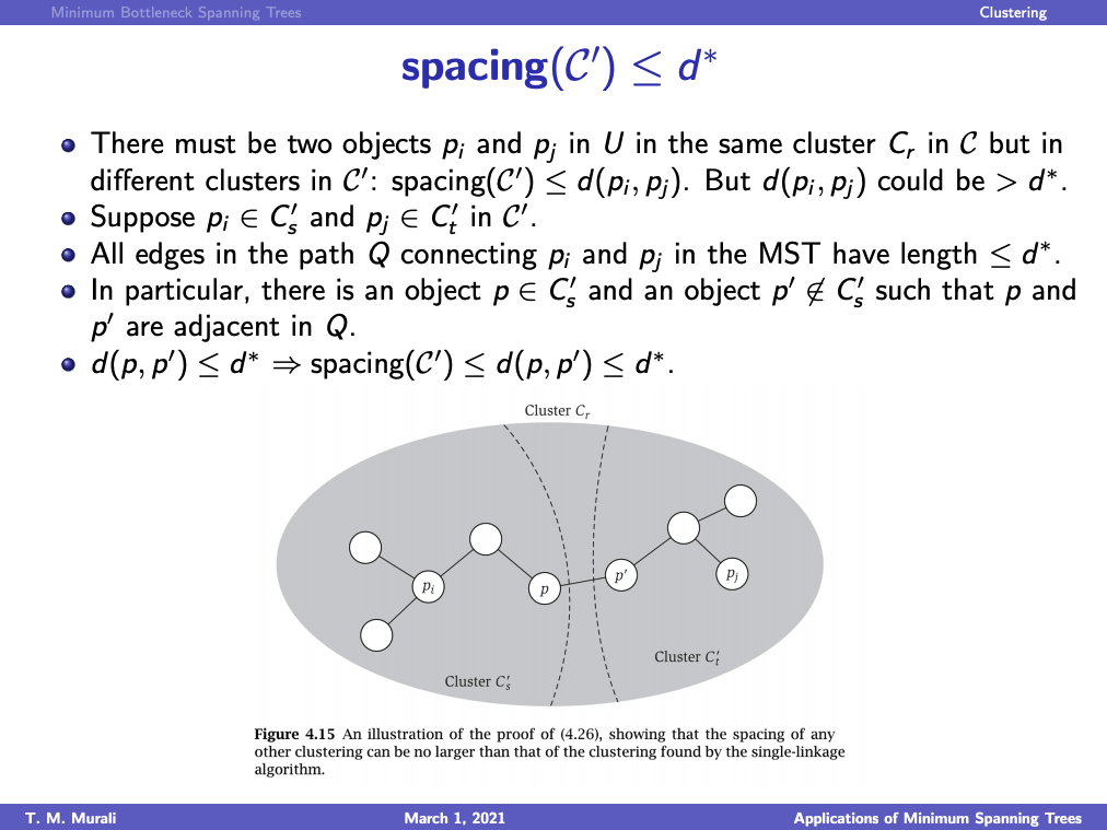
Proof of optimal computing
- Let be any other cluster (with clusters).
- We will prove that spacing()
- There must be two objects in the same cluster but in different clusters in : spacing()
- Suppose and in
- All edges in the path connecting in the MST have lengths
- In particular, there is an object and an object s.t. and are adjacent in
- spacing()
Explanation
- is the name we give to the variable denoting the spacing produced by our algorithm$
- The above proof shows that any other clustering will have a smaller spacing

08 - Divide and Conquer Algorithms
Mergesort
- Instance: nonempty list integers
- Solution: A permutation of such that for all
- Mergesort is a divide and conquer algorithm for sorting
- Partition into two lists of sizes
- Recursively sort ,
- Merge the sorted lists into a sorted list
Merging Two Sorted Lists
- Maintain a current pointer for each list
- initialize each pointed to the front of the list
- While both lists are non-empty:
- let be the elements pointed to by each pointer
- append the smaller of the two to the output list
- advance the current pointer in the list that the smaller element belonged to
- append the rest of the non-empty list to the output
- Running time of this algorithm is ,
Analysing Mergesort
- Running time for = running time for running time for time to split the input into two lists time to merge two sorted lists
- what is this in the worst case?
- worst case running time for time to split input into two lists + time to merge two sorted lists
- This sucks to read, need a shorthand. Let's assume is a power of 2
- Let be the worst-case running time for elements,
- Worst-case running time:
- , is some constant time to split the list
- Can assume for problem sets
Analysing Mergesort in the Worst Case
- Partition into two lists and of size respectively
- Recursively sort and
- Merge the sorted lists into a single sorted list
- Worst case running time for elements ≤
- worst case running time for +
- worst case running time for +
- time to split the input into two lists +
- time to merge two sorted lists
- Assuming is a power of 2:
- Three basic ways of solving this recurrence relation:
- "Unrolling" the recurrence
- Guess a solution and substitute into recurrence to check
- Guess a solution in form and substitute into recurrence to determine the constants
Unrolling

- Input to each sub problem on level has size
- Recursion tree has levels
- Number of sub-problems on level has size
- Total work done at each level is
- Running time of the algorithm is
Substituting a Solution into the Recurrence
Guess that the solution is (log base 2)
Use induction to check if the solution satisfies the recurrence relation
Base case: . Is ? yes.
(strong) Inductive Hypothesis: must include
- Assume , for all , therefore
Inductive Step: Prove
Why is a "loose" bound?
Why doesn't an attempt to prove , for some work?
- (strong) Inductive Hypothesis: must include
- Assume , for all , therefore
- Inductive Step: Prove
what about : it breaks down (I guess?)
Partial Substitution
- (strong) Inductive Hypothesis: must include
Guess that the solution is
Substitute guess into the recurrence relation to check what value of will satisfy the recurrence relation
will work
Proof for all Value of
- We assumed that is a power of 2
- How do we generalize the proof?
- Basic axiom: , for all : worst case running time increase as input size increases
- Let be the smallest power of 2 larger than
- O(n \log n)m \leq 2n$
Other Recurrence Relations
Divide into sub-problems of size and merge in time
two distinct cases:
Divide into two subproblems of size and merge in time
Consider: (finding the median in a set of data)
- Each invocation reduces the problem by a factor of 2 -> there are levels in the recursion tree
- At level of the tree, the problem size is and the work done is
- Therefore the total work done is
since
What about : ?
levels in the recursion tree
At level of the tree, there are sub problems, each of size
Total work done at level is , therefore the total work is
Counting Inversions
Motivation:
- collaborative filtering - match one user's preferences to those of other users
- Meta-search engines - merge results of multiple search engines into a better search results
Two rankings of things are very similar if they have few inversions
- Two rankings have an inversion if there exists such that but
- the number of inversions is a measure of the difference between the rankings
Kendall's rank correlation of two lists of numbers is
Instance: A list of distinct integers between
Solution: The number of pairs s.t.
How many inversions can there be in a list of numbers?
- since every inversion involves a pair of two numbers
Sorting removes all inversion in time. Can we modify mergesort to count inversions?
Candidate algorithm:
- Partition into of size each
- Recursively count the number of inversions in and sort
- Recursively count the number of inversions in and sort
- Count to number of inversions involving on element in and one element in
"Conquer" step
- Given lists and , compute the number of pairs and s.t.
- This step is much easier if are sorted
- Merge-And-Count Procedure:
- Maintain a
currentpointer for each list - Maintain a variable
countinitialized to 0 - Initialize each pointer to the front of each list
- While both lists are non-empty
- Let be the elements pointed to by the
currentpointers - Append the smaller of the two to the output list
- Do something clever in time --> if then
count += m - i, since every element following will also be an inversion with - Advance the
currentpointer of the list containing the smaller list
- Let be the elements pointed to by the
- Append the rest of the non-empty list to the output
- Return
countand the merged list
- Maintain a
Sort and Count
Proof of Correctness
- Proof by induction: Strategy
- a) every inversion in the data is counted exactly once
- b) no non-inversions are counted
- Base case:
- Inductive Hypothesis: Algorithm counts number of inversion correctly for all sets of or fewer numbers
- Inductive Step: Consider an arbitrary inversion, i.e., any pair such that but . When is this inversion counted by the algorithm
- , counted in but the inductive hypothesis
- , counted in but the inductive hypothesis
- . Is this inversion counted by Merge-And-Count? Yes: when is output to the final list is when we count this inversion
- Why is no non-inversion counted? When is output, it is smaller than all remaining elements in since is sorted
09 - Dynamic Programming
Motivation
- Goal: design efficient polynomial time algs
- Greedy:
- pro: natural approach to algorithm design
- con: many greedy approaches; only some may work
- con: many problems for which no greedy approach is known
- Divide and conquer
- pro: simple to develop algorithm skeleton
- con: conquer step can be very hard to implement efficiently
- con: usually reduces time for a problem known to be solvable in polynomial time
- Dynamic Programming
- more powerful than greedy and divide and conquer strategies
- implicitly explore the space of all possible solutions
- solve multiple sub-problems and build up correct solutions to larger and larger subproblems
- careful analysis needed to ensure number of sub-problems solved is polynomial in the size of the input
Example: Greedy Scheduling, but using a DP approach
- Input: start and end time of day: Set
- Constraint: cannot be in two places at one time
- Goal: maximum number of rides you can go on: largest subset of mutually compatible jobs
- EFT: sort jobs in order of increasing finish time, and add compatible jobs to the set
- Use DP to solve a Weighted Interval Scheduling problem:
- Instance: nonempty set and a weight associated with each job
- Solution: A set of mutually compatible jobs such that the value is maximized
- Greedy algorithm can produce arbitrarily bad results for this problem depending on weights
Detour: Binomial Identity
1
1 1
1 2 1
1 3 3 1
- sum of a row =
- Value of a cell in row =
- each element is the sum of the two elements above it
Approach
- Sort jobs in increasing order of finish time and relabel:
- Job comes before job if
- is the largest index such that job is compatible with job
- if there is no such job
- All jobs that come before are also compatible with job

Sub-problems
- Let be the optimal solution: it contains a subset of the input jobs. Two cases to consider:
- Case 1: Job is not in .
- must be the optimal solution for jobs
- Case 2: Job is in
- cannot use incompatible jobs
- Remaining jobs in must be the optimal solution for jobs
- One of the two cases must be true: is the best of the two choices
- Suggests finding optimal solution for sub-problems consisting of jobs , for all values of
- Case 1: Job is not in .
Recursion
- Let be the optimal solution for jobs (a set of jobs) and be the value of this solution:
- We are sooking with a value of , but we start with $j4
- To compute :
- Case 1: :
- Case 2: : //
- When does job belong to ?
- Iff

Running Time of Recusrive Algorithm
- It can be exponential in when : recursive calls are for
- Slide
- However, the same sub-problems get used over and over again, we can cache them
Memoisation
- Store values in a cache using
m_compute_opt(j)and reuse them rather than compute them:
- Claim: running time of algorithm is after sorting
- Time spent in a single call to M-Compute-Opt is apart from time spent in recursive calls
- Total time spent is the order of the number of recursive calls to M-Compute-Opt
- How many such recursive calls are there in total?
- Use number of filled entries in as a measure of progress
- Each time M-Compute-Opt issues two recursive calls, it fills in a new entry in
- Therefore, total number of recursive calls is
Computing in addition to
- explicitly soted in addition to
- Recall: request belong to iff
- Can recover from values of optimal solutions in time
From Recursion to Iteration
- Unwind the recursion and convert it into iteration
- Can compute values of iteratively in time
- Find solution works as before
Basic Outline of Dynamic Programming
- need a collection of sub-problems that satisfy a few properties
- There are a polynomial number of sub problems
- The solution to the problem can by computed easily from the solutions to the sub problems
- There is a natural ordering from "smallest" to "largest"
- There is an easy to compute recurrence that allows us to compute the solution to the sub-problems from solutions to some smaller sub problems
Least Squares Problem
- Given a set of scientific or statistical data plotted on two axes, find the best line that passes through these points
- Instance: Set of points
- Solution: Line that minimizes Error(L,P)
- How many unknown parameters must we find values for?
- via Lagrangian
- and
Segmented Least Squares
Want to fit multiple lines through
Each line must fit contiguous set of x-coordinates
Lines must minimize total error
Divide the points into segments; each segment contains a consecutive set of points ordered by increasing x-coordinate
Instance: Set of points, and a parameter
Solution
- an integer
- a partition of into segments
- for each segment , the best fit line that minimises the total error
if is very large then one line works, if is small, then we fit many lines
How many unknown parameters here? since we need to find the slope and intercept of lines as well a the optimal value of itself
Formulating the Recursion
Let denote the minimum error of a (single) line that fits
Let be the optimal total error for the points
We want to compute
Observation: Where does the last segment in the optimal solution end? , and this segment starts at some point . So the rest of the solution must be the optimal fit for points up to :
is the error for the line that goes through points plus the penalty for adding a line plus the best solution for the last points
If the last segment in the optimal solution is , then
Suppose we want to solve the sub-problem on the first points: : we want to compute
If the last swgment in the optimal partition is then
But can take only distinct values: therefore:
Segment OPT(j) is obtained using index
DP Algorithm
- Computing takes
Let be the running time of this algorithm ( since we compute segments)
RNA Molecules
- basic biological molecule. Single stranded
- RNA molecules fold into complex "secondary structures"
- Secondary structure governs the behavior of an RNA molecule
- carious rules govern secondary structure formation
- Pairs of bases match up; each base matches with ≤ 1 other base
- Adenine : Uracil
- Cytosine : Guanine
- There are no kinks in the folded molecule
- Structures are "knot-free"
- High level problem: given an RNA molecule, predict its secondary structure
Formulating the Problem
- an RNA Molecule is a string ; each
- A secondary structure on is a set of pairs where and
- No kinks: if then
- Watson Crick: The elements in each pair of consist of either or
- is a matching: no index appears in more than one pair
- No knots: If and are two pairs in , then we cannot have
- The Energy of a secondary structure the number of base pairs in it.
- Problem: Compute the largest secondary structure, i.e. with the largest number of base pairs
Dynamic Programming Approach
- is the maximum number of base pairs in a secondary structure for ,
- In the optimal secondary structure on
- If is not a member of any pair, use
- If pairs with some , then the knot condition yields tow independent sub-problems: , ???
- Note that we need that sub-problems to be indexed by both start and by end
- is the maximum number of base pairs in a secondary structure for ,
- In the optimal secondary structure on
- If is not a member of any pair, compute
- If pairs with somme , compute and
- In the "inner" maximization, runs over all indices between that are allowed to pair with
- There are sub-problems: we have a matrix of with the lower right triangle filled out: since the inner summation is less than which we then sum another times
- How do we order them from "smallest" to "largest"? increasing order of
- Note that computing ? : involves sub-problems where
- Total running time for the algorithm is
Dynamic Programming for Shortest Path
Motivation
- Computational finance
- Each node is a financial agent
- The cost of an edge is the cost of a transaction in which we buy from agent and sell to agent
- Negative cost corresponds to profit
- Internet routing protocols
- Dijkstra's algorithm needs knowledge of the entire network
- Routers only know which other routers they are connected to
- Algorithm for shortest paths with negative edges is decentralized
- Not covered in class, but described in Chapter 6.9
Problem Statement
- Input: a directed graph with a cost function i.e., is the cost of the edge
- A negative cycle is a directed graph whose edges have a total cost that is negative
- Two related problems:
- If has no negative cycles, find the shortest s-t path: a path from source to destination with minimum total cost
- Does have a negative cycle?

Approaches for Shortest Path Algorithm
- Dijkstra's
- Computes incorrect answers because it is greedy
- Add some largest constant to each edge
- Computes incorrect answers because the minimum cost path changes
DP Approach
- Assume has no negative cycles
- Claim: there is a shortest path from to that is simple (does not repeat a node) and therefore has at most edges
- How do we define sub-problems?
- Proof: The portion of the path between the two appearances of the node must have a positive cost
- Shortest path has edges: how can we reach using edges, for different values of ?
- We do not know which nodes will be in shortest path: how we can reach from each node in
- Sub-problems defined by varying the number of edges in the shortest path and by varying the starting node in the shortest path
DP Recursion
- : minimum cost of a path that uses at most edges
- is not explicitly mentioned in the sub-problems
- Goal is to compute
- Let be the optimal path whose cost is
- If actually uses edges, then
- If first node on is , then
Alternate DP Formulation
- : minimum cost of a path that uses exactly edges
- a bit harder, but it's in the slides
Bellman-Ford Algorithm
- space used is , running time is
- If shortest path uses edges, we can recover it in time by tracing back through smaller sub-problems
An Improved Bound on the Running Time
- Suppose has nodes and edges. Can we demonstrate a better upper bound on the running time
- only needs to range over outgoing neighbors of
- if is the number of outgoing neighbors of , then in each round, we spend time equal to
- So the total running time can be improved to
Improving the Memory Requirements
- Algorithm still uses space to store the 2D array
- However, depends only on and no other indices
- Modified algorithm:
- Maintain two arrays and indexed over
- At the beginning of each iteration, copy into
- To update , we use
- claim: at the beginning of iteration , stores values of for all nodes
- space used is
Computing the Shortest Path: Algorithm
- How can we recover the shortest path that has cose ?
- For each node , compute and update , the first node after in the current shortest path from to
- Updating : If is the node that attains the minimum in and , set
- At the end, follow points from (and hope for the best lol??)
Computing the Shortest Path: Correctness
- Pointer graph : each edge in is
- Can have cycles?
- is there a path from in ?
- Can there be multiple paths in ?
- Which of these is the shortest path?
Computing the Shortest Path: Cycles in
- Claim: If has a cycle , then has negative cost.
- Suppose we set , at this instant
- Comparing and , we know that
- Between this assignment and the assignment of to some other node, may itself decrease. Hence, , in general
- Let be the nodes in and assume that is the last edge to have been added.
- What is the situation just before this addition?
- for all ,
- Adding all these inequalities: cost of
- Corollary: if has no negative cycles then does not either
Computing the Shortest Path: Paths in
- Let be the pointer graph upon termination of the algorithm
- Consider the path in obtained by following the pointers from to to and so on
- Claim: terminates at
- Claim is the shortest path in from to
Bellman-For algorithm: One Array
- In general, after iterations, the path whose length is may have many more than edges
- Early termination: if does not change after processing all the nodes, we have computed all shortest paths to
10 - Network Flow
Motivation
- Fundamental problems in combinatorial optimization
- duality between flow and cuts
Flow Networks
- Use directed graphs to model transport networks:
- edges carry traffic and have capacities
- nodes act as switches
- source nodes generate traffic, sink nodes absorb traffic
- A flow network is a directed graph
- each edge has a capacity
- There is a single source node
- There is a single sink node
- Nodes other than are internal
Defining Flow
- In a flow network , an flow is a function such that:
- (Capacity conditions) for each
- (Conservation conditions) for each internal node ,
- The value of a flow is
Maximum-Flow Problem
- Instance: a flow network
- Solution: The flow with the largest value in , where the maximum is taking over all possible flows on
- Output should assign a flow value to each edge in the graph
- The flow on each edge should satisfy the capacity condition
- The flow into and out of each internal node should satisfy the conservation conditions
- the value of the output flow, i.e., the total flow out of the source node in the output flow, must be the largest possible over all possible flows in
- Assumptions:
- Node edges enter , no edges leave
- There is at least one edge incident on each node
- all edge capacities are integers
Developing the Algorithm
- No known DP algorithm
- Greedy approach instead
- Start with zero flow along all edges
- find an path and push as much flow along it as possible
- idea is to increase flow: push flow along edges with leftover capacity and undow flow along edges already carrying flow
Residual graph
- Give a flow network and a flow on , the residual graph of w.r.t. is a directed graph such that:
- (Nodes) has the same nodes as
- (Forward edges) for each edge s.t. , contains the edge with a residual capacity
- (Backward edges) for each edge s.t. , contains the edge with a residual capacity
Augmenting Paths in a Residual graph
- Let be a simple path in
- is the minimum residual capacity of any edge in
- is forward in iff flow increases along
- is backward in iff flow decreases along
Correctness of
- A simple path in the residual graph is an augmenting path
- Let be the flow returned by
- Claim: is a flow. Verify capacity and conservation conditions
- Only need to check edges and internal nodes in
- Capacity condition on : note that residual capacity of
- is a forward edge:

- is a backward edge:

- Conservation condition on internal node – four cases to work out:

Ford-Fulkerson Algorithm
- Does it terminate? What is it doing?


We can see here, the max flow path is , with a bottleneck of along, that edge gets augmented
Repeat
Analysis of the Ford-Faulkerson Algorithm
- Running time:
- Does it terminate? If so, how many loops, since each loop is
- Claim at each stage, flow values and residual capacities are integers. Prove by induction
- Claim: Flow value strictly increase when we apply
- recall every edge that is incident on is a forward edge
- the flow along these edges will increase by
- Claim : Maximum value of any flow
- Claim: Algorithm terminates in at most iterations
- Claim: Algorithm runs in time
Correctness of the Ford-Faulkerson Algorithm
- How large can the flow be?
- Can we characterize the magnitude of the flow in terms of the structure of the graph? For example, for every flow
- Is there a better bound?
- Proof strategy:
- Define cut, its capacity, and flow in and out of the cut
- For any cut, prove any flow its capacity
- Define a specific cut at the end of the Ford-Faulkerson algorithm
- Prove that the flow across this cut equals its capacity
Cuts and Capacities
- An cut is a partition of into sets and such that and
- Capacity of the is
- Intuition: For every flow


Fun Facts about Cuts
- Let be any flow and any cut
- Claim:
- and
- For ever other node ,
- Summing up all these equations,
- An edge that has both ends in or both ends out of does not contribute
- An edge that has its tail in contributes
- An edge that has its head in contributes
- Corollary:
Important Fact about Cuts
Max-Flows and Min-Cuts
- Let be any flow and any cut. We proved
- Very strong statement: The value of every flow is capacity of any cut
- Corollary: The maximum flow is at most the smallest capacity of a cut
- Question: Is the reverse true? Is the smallest capacity of a cut at most the maximum flow
- Answer: Yes, the Ford-Faulkerson algorithm computes this cut!
Flows and Cuts
- Let denote the flow computed by the Ford-Faulkerson algorithm
- Enough to show cut such that
- When the algorithm terminates, the residual graph has no path
- Claim: If is an flow such that has no path, then there is an cut such that
- Claim applies to any flow such that has no path, and not just to the flow computed by the Ford-Faulkerson algorithm
Proof of Claim Relating Flows to Cuts
- Claim: is an flow and has no path cut
- set of nodes reachable from in
- Claim: is an cut in
- Claim: If such that , then
- Claim: If such that , then
- Claim
Max-Flow Min-Cut Theorem
- The flow computed by the Ford-Faulkerson algorithm is a maximum flow
- Given a flow of maximum value, we can compute a minimum cut in time
- In every flow network, there is a flow and a cut such that
- Max-Flow Min-Cut Theorem: in every flow network, the maximum value of an flow is equal to the minimum capacity of an cut
- Corollary: If all capacities in a flow network are integers, then there is a maximum flow where , the value of the flow on edge , is an integer for every edge
Real-Valued Capacities
- If capacities are real-valued, Ford-Faulkerson algorithm may not terminate!
- But Max-Flow Min-Cut theorem is still true, why?
Improving Ford-Faulkerson Algorithm
- Bad case for Ford-Faulkerson is when the bottleneck edge is the augmenting path has a low capacity
- Idea: decrease number of iterations by picking path with bottleneck edge of largest capacity. Computing this path can slow down each iteration considerably.
- Modified idea: Maintain a scaling parameter and choose only augmenting paths with bottleneck capacity at least
- : residual network restricted to edges with residual capacities
11 - Network Flow Applications
Maximum Flow and Minimum Cut Problems
Matching in Bipartite Graphs
- Bipartite Graph a graph where
- are disjoint and
- Bipartite graphs model situations in which objects are matched with or assigned to other objects: e.g. marraiges, residents/hospitals, jobs/machines
- A Matching in a bipartite graph is a set of edges such that each node of is incident on at most edge of
- A set of edges is a perfect matching if every node in is incident on exactly one edge in
- Instance: A bipartite graph
- Solution: The matching of largest size in
Algorithm for Bipartite Graph Matching
- Convert to a flow network : direct edges from to , add nodes and connect to each node in and to each node in , set all edge capacities to 1
- Computer the maximum flow in
- Convert the maximum flow in into a matching in
- Claim: the value of the maximum flow in equals the size of hte maximum matching in
- In general, there is a matching of size in if an only if there is a (integer valued) flow of in
Strategy for Proving Correctness
- Preclude the possibilities that has a flow of value but we cannot construct a matching in with edges
- Matching => flow: if there is a matching with edges in , there is an flow of value in
- How do we construct this flow?
- Consider every edge in the matching:
- Send on unit of flow along the path
- Why have we constructed a flow
- Capacity constraint: No edges receive a flow because we started with a matching
- Conservation constraint: Every node other than and has one incoming unit and one outgoing unit of flow because we started with a matching
- What is the value of the flow? , since exactly that many nodes out of carry flow
Now let us consider the reverse side of the reduction
- Flow => matching: if there is a flow in with value , there is a matching in with edges
- There is an integer-valued flow of value flow along any edge is 0 or 1
- Let be the set of edges not incident on or with flow equal to 1
- Claim: contains edges
- Claim Each node in (respectively, ) is the tail (respectively, head) of at most one edge in
- Conclusion: size of the maximum matching in is equal to the value of the maximum flow in : the edges in this matching are those that carry flow from to in
In general, we must prove that the reduction is bi-directional, or isomorphic
Running time of Bipartite Graph Matching Algorithm
- Suppose has edges in nodes in , and in
- Ford-Fulkerson algorithm runs in time
- How do we determine if a bipartite graph has a perfect matching? Find the maximum matching and check if it is perfect
- Suppose has no perfect matching. Can we exhibit a short "certificate" of that fact? What can such certificates look like?
- has no perfect matching iff there is a cut in with capacity less than . Therefore, the cut is a certificate
- We would like the certificate in terms of
- For example, two nodes in with on incident edge each with the same neighbor in
- Generally, a subset with neighbors , such that
- Hall's Theorem Let be a bipartite graph such that . Then either has a perfect matching or there is a subset such that . We can compute a perfect matching or such a subset in time.
- , the neighbors of
Edge-Disjoint Paths
- A set of paths in a directed graph is edge disjoint if each edge in appears in at most one path
- Instance: Directed graph with two distinguished nodes
- Solution: The maximum number of edge-disjoiint paths between and
Mapping to the Max-Flow Problem
- Convert into a flow network with edge capacities of 1
- Claim: There are edge-disjoint paths from in a directed graph if and only if there is a flow in with value
- Paths => flow: if there are edge-disjoint paths from to , send one unit of flowin along each to yield a flow with value
- Flow => paths: Suppose there is an integer-valued flow of value at least . Are there edge-disjoint paths? If so, what are they?
- There is an integral flow. Therefore flow on each edge is 0, or 1
- Claim: if is a 0-1 value flow of value , the the set of edges with flow contains a set of edge-disjoint paths
- But how do we show that this set of edges with flow value of 1 actually form paths?
- Claim if is a valued flow of value m then the set of edges with flow contains a set of edge-disjoint paths
- Prove by induction on the number of edges in that carry flow. Let this number be .
- Base case: . Nothing to prove
- Inductive Hypothesis: For every flow in with
- value carrying flow on edges or
- value carrying flow on edges, the set of edges with contains a set of edge-disjoint paths
- Inductive Step: Construct a set of paths from . Work out by hand
- Note: formulating the inductive hypothesis can be trick
- Strategy is to prove the inductive step first
- During this proof, we observe two types of "smaller" flows:
- When you succeed in finding an path, we get a new flow that is smaller, i.e. carrying flow on fewer edges, i.e.
- When we run into a cycle, we get a new flow with but carrying flow on fewer edges, i.e.
- We combine both situations in the inductive hypothesis
Certificate for Edge-Disjoint Paths Algorithm
- A set of edges separatees if the graph contains no paths
- Menger's Theorem: In every directed graph with nodes , the maximum number of edge disjoint paths is equal to the minimum number of edges whose removal disconnes from .
Running Time of the Edge-Disjoint Paths Algorithm
- Given a flow of value , how quickly can we determine the edge-disjoint paths?
- Corollary: The Ford-Fulkerson algorithm can be used to find a maximum set of edge-disjoint paths in a directed graph in time.
Edge-Disjoint Paths in Undirected Graphs
- Can extend the theorem to undirected graphs
- Replace each edge with two directed edges of capacity 1 and apply the algorithm for directed graphs
- Problem: Both counterparts of an undirected edge may be used by differnt edge-disjoint paths on the directed graph
- resolved by zeroing out flow for edges where flow goes in both directions
- Can obtain an integral flow where only one of the directed counterparts of has non-zero flow
- We can find the maximum number of edge disjoint paths in time
- We can prove a version of Menger's theorem for undirected graphs: in every undirected graph with nodes , the maximum number of edge-disjoint paths is equal to the minimum number of edges whose removal separates from
Image Segmentation
- Fundemental problem in computer vision: segmentaing an image into coherent regions
- A basic segmentation problem is that of partitioning an image into a foreground and a background: label each pixel in the image as belonging to one of those two
- Let be the set of pixels in an image
- Let be the set of pairs of neighboring pixels
- and yield an undirected graph
- Each pixel has a likelihood that it belongs to the foreground and a likelihood that it belongs to the background
- These likelihoods are specified in the input to the problem
- We want to fg/bg boundary to be smooth: for each pait of pixels, there is a separation penalty for placing one of them in the foreground and the other in the background
Formulating the Problem
- Instance: Pixel graphs , likelihood functions , penalty function
- Solution: Optimum labelling: partition of the pixels into two sets that maximizes
- There is a similarity between cuts and labellings
- Differences:
- Maximizing an objective function rather than minimizing
- There is no source or sink in the segmentation problem
- We have values on the nodes
- The graph is undirected
Maximization to Minimization
- Let
- Notice that
- Therefore, maximizing
is identical to minimizing
Solving the Other Issues
- Solve the other issues like we did earlier:
- Add a new "super-source" to represent foreground
- Add a new "super-sink" to represent the background
- Connect to every pixel and assign capacity to edge and capacity to edge
- Direct edges away from and into
- Replace each edge in with two directed edges of capacity
- Now we want the minimum capacity cut
Cuts in the Flow Network
- Let be this flow network and and cut
- What does the capacity of the cut represent?
- Edges crossing the cut can be one of three types:
- contributes to
- contributes to
- contributes to
- So, the capacity of an cut exactly measure the quantity
- To maximise , we compute the cut of minimum capacity
- Deleting from the cut yields the desired segmentation of the image
- Thus, Image Segmentation is reduced to a Minimum Cut problem
12 - NP and Computational Intractibility
Algorithm Design
- Patterns:
- Greed interval scheduling
- Divide and Conquer counting inversions
- Dynamic Programmming RNA folding
- Duality: maximum flow and minimum cuts
- Reductions
- Local search
- Randomization
- Anti-Patterns
- NP-completeness: algorithm unlikely
- PSPACE-completeness: certification algorithm unlikely
- Undecidability: no algorithm possible
Computational Tractability
- When is an algorithm an efficient solution to a problem? When the running time is polynomial in the size of the input
- A problem is computationally tractable if it has a polynomial time algorithm solution
| Polynomial time | Probably not |
|---|---|
| Shortest path | Longest Path |
| Matching | 3D Matching |
| Min cut | Max cut |
| 2-SAT | 3 SAT |
| Planar four-color | Planar 3 color |
| Bipartite vertex cover | vertex cover |
| Primarily testing | Factoring |
Problem Classification
- Classify problems based on whether they admit efficient solutions or not
- Some extremely hard problems cannot be solved efficiently (e.g. chess on an board)
- However, classification is unclear for a large number of problems
- We can prove that these problems are fundementally equivalent and are manifestations of the same problem!
Polynomial-Time Reduction
- Goal is to express statements of the type: "Problem X is at least as hard as problem Y"
- Use the notion of reductions
- Y is polynomial-time reducible to if any arbitrary instance (input) of can be solved using a polynomial number of standard operations, plus one call to a black box that solves problem
- Maximum Bipartite Matching Maxmum Flow
- Maximum Bipartite Matching Maxmum Flow because you can't reduce a network flow to a bipartite matching...
- You can get 4 from 3 by adding 1, but you can't get 3 from 4 by adding 1
- Image Segmentation Minimum Cut
- polynomial time reducable
- Maximum Bipartite Matching Maxmum Flow
- implies that " is at least as hard as "
- Such reductions are Karp reductions. Cook reductions allow a polynomial number of calls to the black box that solves
Usefulness of Reductions
- Claim: If and can be solved in polynomial time, then can be solved in polynomial time
- Contrapositive: If and cannot be solved in polynomial time, then cannot be solved in polynomial time
- Informally: If is hard, and we can show that reduces to , then the hardness "spreads" to
Reduction Strategies
Simple equivalence
Special case to general case
Encoding with gadgets
Optimisiation versus Decision Problems
- So far, we have developed algorithms that solve optimisation problems
- Compute the largest flow
- Find the closest pair of points
- Find the schedule with the least completion time
- Now, we turn our attention to decision versions of problems, e.g. is there a flow with value at least , for a given value of
- Decision problem: answer to every input is yes or no
Primes
- Instance: A natural number
- Question: Is prime?
Independent Set and Vertex Cover
- Given an undirected graph , a subset is an independent set if no two vertices in are connected by an edge
- Instance: Undirected graph and an integer
- Question: Does contain an independent set of size
- Given an undirected graph , a subset is a vertex cover if every edge in is incident on at least one vertex in
- Instance: Undirected graph and an integer
- Question: Does contain a vertx cover of size
- Goal: Demonstrate a simple equivalence between these two problems
- Claim: Independent Set Vertex Cover and Vertex Cover Independent Set
- N.B. the inverse of an independent set must be a vertex cover
Strategy for Proving Independent Set Vertex Cover
- Start with an arbitrary instance of IS: an undirected graph and an integer
- From and , create an instance of VC: an undirected graph and an integer
- is related to in some way
- can depend upon and size of
- Prove that has an IS of size iff has a vertex cover of size
- Transformation and proof must be correct for all possible graphs and all possible values of
- This proof is an iff because we're using a blackbox algorithm for VC to solve IS
- If there is an independent set size , we must be sure that there is a vertex cover of size , so that we know that the black box will find this vertex cover
- If the black box finds a vertex cover of size , we must be sure we can construct an independent set of size from this vertex cover
- This proof is an iff because we're using a blackbox algorithm for VC to solve IS
- Arbitrary instance of IS:
- Let
- Create an instance of VC:
- Claim: has an IS of size iff has a VC of size
- Proof: is an IS in iff is a VC in G
- The same idea proces that VC IS
Vertex Cover and Set Cover
- IS is a "packing" problem: pack as many vertices as possible, subject to constraints (the edges)
- VC is a "covering" problem: cover all edges in the graph with as few vertices as possible
Microbe Cover
- Instance: A set of compounds, a collection of microbes, where each microbe can make a subset of compounds in , and an integer
- Question: Is there a subset of microbes that can together make all the compounds in ?

Vertex Cover Microbe Cover

- Input to VC: an undirected graph and an integer
- Let
- Create an instance of Microbe cover where:
- , i.e. each element of is an edge of
- For each node , create a microbe whose compounds are the set of edges incident on
- Claim: can be covered with microbes iff has a VC cover with nodes
- Proof strategy:
- If has a VC of size , then can be covered with
- If can be covered with microbes, then has a vertex cover of size
- this is a different form of the Set Cover problem:
- Instance: A set of elements, a collection of subsets of , and an integer
- Question: Is there a collection of sets in the collections whose union is ?
Boolean Satisfiability
- Abstract problems formulated in Boolean notation
- given a set of Boolean variables
- Each term can take the value of
- Term: a variable or its negation
- Cause of Length: (or) distinct terms
- Truth assignment for : is a function
- An assignment satisfies a clause if it causes at least one term in to evaluate to 1 (since is an or of terms)
- An assignment satisfies a collection of clauses if it causes all clauses to evaluate to 1 i.e.
- is a satisfying assignment with respect to
- set of clauses is satisfiable
Examples
- Terms:
- Clauses:
- Assignment:
- Not satisfying because of clauses 1, 3
- Assignment:
- is satisfying
SAT and 3-SAT
- Instance: A set of clauses , each of length 3, over a set of variables
- Question: IS there a satisfying truth assignment for with respect to
- SAT and 3-SAT are fundemental combinatorial search problems
- We have to make independent decisions (the assignments for each variable) while satisfying the set constrains
- Satisfying each constraint in isolation is easy, but we have to make our decision so that all constraints are satisfied simultanesouly
Example
Clauses:
- Is satisfiable? Yes by
- Is satisfiable? Yes by
- Is satisfiable? Yes by
- Is satisfiable? No
3-SAT Independent set
- Two ways to think about 3-SAT:
- Make an independent 0/1 decision on each variable and succeed if we achieve on of three ways in which to satisfy each clause
- Choose (at least) one term from each clause. Find a truth assignment that causes each chose term to evaluate to 1. Ensure that no two terms selected conflict e.g. select in and in
- We are given an instance of 3-SAT with clauses of length three over variables

- Construct an instance of Independent Set: graph with nodes
- For each clause , add a triangle of three nodes and three edges to
- Label each node with the th term in
- Add an edge between each pair of nodes whose labels correspond to terms that conflict
- N.B. size of largest IS is
- can be assigned either 0 or 1 to satisfy the clauses.
- Claim: 3-SAT instance is satisfiable iff has an independent set of size
- Satisfiable assignment Independent Set of size : Each triangle in has at least one node whose label evaluates to 1. Set of nodes consisteing of one such node from each triangle forms an independent set of size = . Why?
- Independent Set of size Satisfiable assignment: the size of this set is . How do we construct a ssatisfying truth assignment from the nodes in the independent set?
- For each variable , only or is the label of a node in .
- If is the label of a node in , set ; else set
Transitivity of Reductions
- Claim: If and , than
- Note that If , then ? False
- We have shown that 3-SAT Independent Set Vertex Covert Set Cover
Finding vs. Certifying
- Is it easy to check if a given set of vertices in an undirected graph forms an independent set of size at least
- Is it east to check if a particular truth assignment satisfies a set of clauses?
- We draw a contrast between finding a solution and checking a solution (in polynomial time)
- Since we have not been able to develop efficient algorithms to solve many decision problems, let us turn our attention to whether we can check if a proposed solution is correct
Problems and Algorithms
Primes
- Instance: A natural number
- Question: Is prime?
- Decision problem : for every input answer is yes or no
- An algorithm for a decision problem receives an input and returns
- An algorithm solves the problem if for every input
- if then and
- if then
- has a polynomial running time if there is a polynomial function such that for every input , terminates on in at most steps
- There is an algorithm such that for the Primes problem, improved to
- : is a set of problems for which there is a polynomial time algorithm
- A decision problem is in iff there is an algorithm with polynomial running time that solves
Efficient Certification
- A "checking" algorithm for a decision problem has a different structure from an algorithm that solves
- Checking an algorithm needs input as well as a separate "certificate" that contain evidence that
- An algorithm is an efficient certifier for a problem if
- is a polynomial time algorithm that takes two inputs and
- for all inputs : - iff there is a certificate such that , and - the size of is polynomial in the size of
- Certifier's job is to take a candidate certificate that and check in polynomial time whether is a correct certififcate
- Certificate must be "short" so that certifier can run in polynomial time
- Certifier does not care about how to find these certificates
- : Set of problems for which there is a polynomial time algorithm
- : Set of all problems for which there exists an efficient certifier
- 3-SAT
- Certificate : a truth assignment to the variables
- Certifier : checks whether the assignment causes every clause to evaluate to true
- Independent set
- Certificate : a set of at least vertices
- Certifier : checks that no pair of vertices are connected by an edge
- Set Cover :
- Certificate : a list of sets from the collection
- Certifier : checks if the union of these sets is
vs.
- Claim:
- Let be any problem in
- There is a polynomial time algorithm that solves
- ignores and simply returns . Why is an efficient certifier
- just has to check the certificate, not compute it
- Is or is . Major unsolved problem in CS
Summary
- 3-SAT, Vertex Cover, Set Cover, Independent Set are in
- 3-SAT Independent Set Vertex Cover Set Cover
- What is the structure of the problems in
- Is there a sequence of problems in , such that
- Are there two problems and in such that there is no problem such that there is no problem
-Complete and -Hard problems
A problem is -Complete if
- and
- for every problem
A problem is -Hard if
- for every problem
Claim: Suppose is -Complete, then iff
Corollary: If there is any problem in that cannot be solved in polynomial time, then no -Complete problem can be solved in polynomial time
Does even one -Complete problem exist?! If it does, how can we prove that every problem in reduces to this problem
Circuit Satisfiability
- Cook-Levin Theorem: Circuit Satisfiability is -Complete
- A circuit is a labelled, directed acyclic graph such that
- the sources in are labelled with constants (0 or 1) or the name of a distinct variable (the inputs of the circuit)
- every other node is labeled with one Boolean operator
- a single node with not outgoing edges represents the output of
- Instance: A circuit
- Question: Is there a truth assignment to the inputs that causes the output to have value 1?
13 - NP-Complete Problems
Proving Other Problems -Complete
- Claim: If is -Complete and such that , then is -Complete
- Recall that is -Complete if
- is in and
- for every problem in ,
- Given a new problem , a general strategy for proving it -Complete is
- Prove that
- Select a problem known to be -Complete
- Prove that
3-SAT is -Complete
- Why is 3-SAT in
- Circuit Satifiability 3-SAT
- Given an input to Circuit Satisfiability, create an input to SAT in which each clause has at most 3 variables
- Convert this input to SAT into an input to 3-SAT
More -Complete Problems
- Circuit Satisfiability is -Complete
- We just show Circuit Satisfiability 3-SAT
- 3-SAT IS VC Set Cover
- All of these problems are in
- Therefore, all -Complete problems are reducible to each other
Hamiltonian Cycle
- Problems we have seen so far involve searching over subsets of a collection of objects
- Another type of computationally hard problem involves searching over the set of all permutations of a collection of objects
- In a directed graph , a cycle is a Hamiltonian Cycle if visits each vertex exactly once
- Instance: A directed graph
- Question: Does contain a Hamiltonian Cycle?
Hamiltonian Cycle is -Complete
- Claim: 3-SAT Hamiltonian Cycle
- Proof coming up
Travelling Salesman Problem
- A salesman must visit cities starting at home city
- Salseman must find a , an order in which to visit each city exactly once and return home
- Goal is to find as short a tour as possible
- For every pair is the distance between them
- a tour is a permutation of
- The length of a tour is
- Instance: A set of cities, a function , anda number
- Question: Is there a tour of length at most
Travelling Salesman is -Complete
- Why is the problem in
- Why is the problem -Complete
- Claim: Hamiltonian Cycle Trevelling Salesman
| HC | TSP |
|---|---|
| Directed Graph | Cities |
| Edges have identical weights | Distance between cities can vary |
| Not all pairs of nodes are connected in | Every pair of cities has a distance |
| and may both be edges |
14 - Coping with NP-Completeness
- These problems come up in real life
- -Complete means that a problem is hard to solve in the worse case. Can we come up with better solutions at least in some cases?
- Develop algorithms that are exponential in one parameter in the problem
- Consider special cases of the input e.g. graphs that "look like" trees
- Develop algorithms that can provably compute a solution close to the optimal
Vertex Cover
- Instance: Undirected graph and an integer
- Question: Does contain a vertex cover of size at most ?
- Problem has two parameters:
- What is the running time of a brute force algorithm:
- Can we devise an algorithm whose running time is exponential in but polynomial in e.g.
- Fixed parameter tractable
Designing the Vertex Cover Algorithm
- Intuition: if a graph has a small Vertex Cover, it cannot have too many edges
- Claim: If has nodes and has a vertex cover of size at most , then has at most edges
- Easy part of algorithm: Return no if has more than edges
- is the graph w/o the node and the edge incident on
- Consier an edge . Either or must be in the vertex cover
- Claim: has a vertex cover of size at most iff for any edge either or has a vertex cover of size at most
Analysing the Vertex Cover Algorithm
- Develop a recurrence relation for the algorithm with parameters
- Let denote the worst-case running time of the algorithm on an instance of Vertex Cover with parameters
- We need time to count the number of edges
- Claim:
Solving -Hard Problems on Trees
- -Hard: at least as hard as -Complete. We use -Hard to refer to optimisation version of decision problems
- Many -Hard problems can be solved efficiently on tree
- Intuition: subtree rooted at any node pf the tree interacts with the rest of the treee only through . Therefore, depending on whether we include in the solution or not, we can decouple solving the problem in 's subtree from the rest of the tree
Approximation Algorithms
- Methods for optimisation version of -Complete Problems
- Run in polynomial time
- Solution returned is guaranteed to be within a small factor of the optimal solution
Approximation Algorithm for Vertex Cover
- Running time is linear on the size of the graph
- Claim: is a vertex cover
- Claim: No two edges in can be covered by the same node
- Claim: The size of the smallest vertex cover is at least
- Claim:
- No approximation algorithm with a factor better than 1.3606 is possible unless (Dinur, Safra 2006)
- No approximation algorithm with a factor better than 2 is possible if the "unique games conjecture" is true (Khot, Regev 2008)
Load Balancing Problem
- Given a set of machines
- Given a set of jobs: job has processing time
- Assign each job to one machine so that the time spent is minimised
- Let be the set of jobs assigned to machine
- Total time spent on machine is
- Minimise makespan , the largest load on any machine
- This is -Complete
Lower Bounds on the Optimal Makespan
- Need a lower bound on the optimum makespan
- The two bound below suffice:
- Claim: computed makespane
- Let be the machine whose load is and be the last job placed on
- What was the situation just before placing this job?
- had the smallest load and its load was
- For every machine , load
Improving the Bound
- It is easy to construct an example for which the greedy algorithm produces a solution close to a factor of 2 away from the optimal
- How can we improve?
- What if we process the jobs in decreasing order of processing time
Analyzing Sorted-Balance
- Claim: if there are fewer than jobs, algorithm is optimal
- Claim: if there are more than jobs, then
- Consider only the first jobs in sorted order
- Consider any assignment of these jobs to machines
- Some machine must be assigned two hobs, each with processing time
- This machine will have a load at least
- Claim:
- Let be the machine whose load is and be the last job placed on ( has at least two jobs)
- There is an even better bound
- polynomial-time approximation scheme: for every , compute solution with makespan in
Partition Problem
- Instance: a set of natural numbers
- Solution: a subset of numbers such that
Subset Sum Problem
- Instance: a set of natural numbers and a target
- Solution: a subset of numbers such that is maximized subject to the constraint
- is the largest sum possible using only the first numbers with target
Running itme is
All of these are -Complete: 3D-Matching Partition Subset Sum Knapsack
Knapsack Problem
- Instance: a set of elements, with each element having a weight and a value , and a knapsack capacity of
- Solution: a subset of items such that is maximized subject to the constraint
Dynamic Programming for Knapsack
- Can generalize the DP program for Subset Sum
- Develop a different DP program that will be useful later
- is the smallest knapsack weight so that there is a solution using only the first items with total value
- What are the ranges of ?
- ranges between , the number of items
- Given ranges between
- Largest value of is where
- The solution we want is the largest value such that
- for every
- , otherwise
- Can find items in the solution by tracing back
- Running time is which is pseudo-polynomial in the input size
Intuition underlying Approximation Algorithm
- What is the running time if all values are the same
- What if they're all small integers
- Idea:
- round and scale all the values to lie in a smaller range
- run the DP algorithm with the modified new values
- Return items in this optimal solution
- prove that the value of this solution is not much smaller than the true optimum
Approximation Scheme for Knapsack
- is a precision parameter: assume that is an integer
- Scaling factor
- for every item , and set:
- algorithm:
- solve knapsack problems using the DP program with the values
- Return the set of items found
- Running time of Knapsack-Approx?
- Have to include here because it determines the size of the input
- We need to show that the value of the solution returned by Knapsack-Approx is good
Approximation Guarantee for Knapsack-Approx
- Let be the solution computed by Knapsack-Approx
- Let be any other solution satisfying
- Claim:
- Since Knapsack-Approx is optimal for the values :
- Since for each ,
- Apply argument to containing only the items with the largest value:
- Therefore
- The running time can be improved to
15 - Solutions
Homework 1
Homework 2
Homework 3
Homework 4
Midterm
Homework 5
Homework 6
Homework 7
Final